Mediation with svyset Data
Current versions of Stata support svy: sem and
estat teffects without complaint. There is
no longer a need to use gsem and manual
calculation. However, this document may still be useful as either a
guide to using estat teffects or manually calculating them
if you need to use gsem for another reason.
Mediation models in Stata are fit with the sem command.
sem does not support svyset data, so instead
you use gsem (e.g. svy: gsem ...).
However, gsem does not support estat teffects
which calculates direct, indirect and total effects.
This document shows how to manually calculate these effects using
nlcom.
Note that this is a case where all variables are continuous and all
models are linear - we are only using gsem for it’s support
of svy:, not it’s support of GLMs. Indirect effects are a
more complicated topic in those models which we do not address here.
Additionally, we’ll trust Stata to compute standard errors rather than
getting into any sticky issues of bootstrapping.
Standard Mediation
First, let’s estimate the direct, indirect and total effects without the use of the survey design to show equivalence.
. webuse gsem_multmed
(Fictional job-performance data)
The model we’ll be fitting is
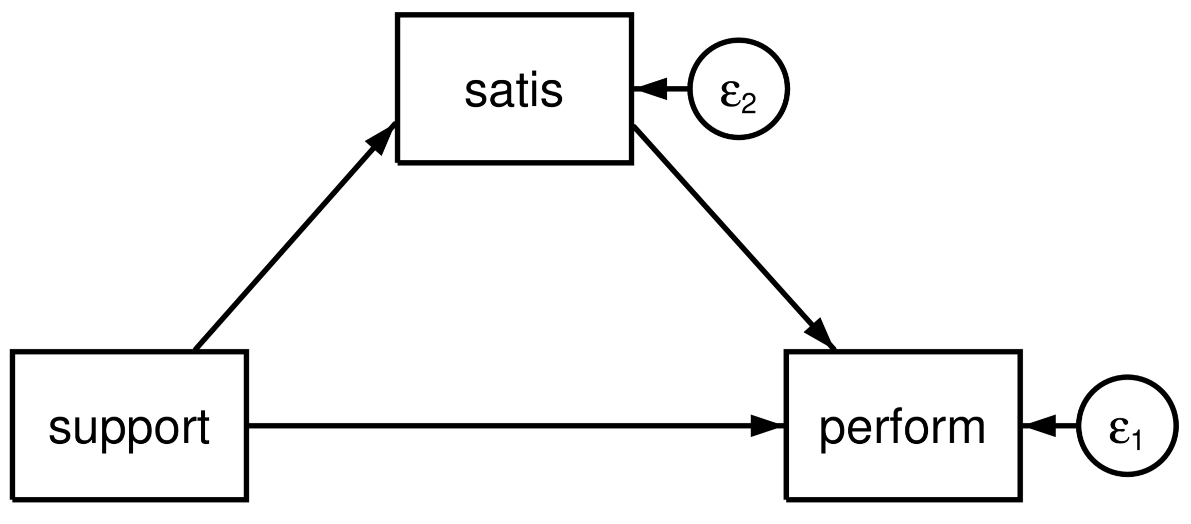
Here, “satis” is a potential mediator between “support” and “perform”. The direct effect is the arrow between “support” and “perform”, the indirect effect is the arrows from “support” to “perform” which passes through “satis”, and the total effect is the sum of the direct and indirect effects.
. sem (perform <- satis support) (satis <- support)

Endogenous variables
  Observed: perform satis

Exogenous variables
  Observed: support

Fitting target model:
Iteration 0:  Log likelihood = -3779.9224
Iteration 1:  Log likelihood = -3779.9224

Structural equation model                                Number of obs = 1,500
Estimation method: ml

Log likelihood = -3779.9224

------------------------------------------------------------------------------
             |                 OIM
             | Coefficient  std. err.      z    P>|z|     [95% conf. interval]
-------------+----------------------------------------------------------------
Structural   |
  perform    |
       satis |   .8984401   .0251903    35.67   0.000      .849068    .9478123
     support |   .6161077   .0303143    20.32   0.000     .5566927    .6755227
       _cons |   4.981054   .0150589   330.77   0.000     4.951539    5.010569
  -----------+----------------------------------------------------------------
  satis      |
     support |   .2288945   .0305047     7.50   0.000     .1691064    .2886826
       _cons |    .019262   .0154273     1.25   0.212    -.0109749    .0494989
-------------+----------------------------------------------------------------
var(e.perf~m)|   .3397087   .0124044                      .3162461     .364912
 var(e.satis)|   .3569007   .0130322                      .3322507    .3833795
------------------------------------------------------------------------------
LR test of model vs. saturated: chi2(0) = 0.00                 Prob > chi2 = .
The direct, indirect and total effects can be estimated via
estat teffects.
. estat teffects


Direct effects
------------------------------------------------------------------------------
             |                 OIM
             | Coefficient  std. err.      z    P>|z|     [95% conf. interval]
-------------+----------------------------------------------------------------
Structural   |
  perform    |
       satis |   .8984401   .0251903    35.67   0.000      .849068    .9478123
     support |   .6161077   .0303143    20.32   0.000     .5566927    .6755227
  -----------+----------------------------------------------------------------
  satis      |
     support |   .2288945   .0305047     7.50   0.000     .1691064    .2886826
------------------------------------------------------------------------------


Indirect effects
------------------------------------------------------------------------------
             |                 OIM
             | Coefficient  std. err.      z    P>|z|     [95% conf. interval]
-------------+----------------------------------------------------------------
Structural   |
  perform    |
       satis |          0  (no path)
     support |    .205648   .0280066     7.34   0.000      .150756      .26054
  -----------+----------------------------------------------------------------
  satis      |
     support |          0  (no path)
------------------------------------------------------------------------------


Total effects
------------------------------------------------------------------------------
             |                 OIM
             | Coefficient  std. err.      z    P>|z|     [95% conf. interval]
-------------+----------------------------------------------------------------
Structural   |
  perform    |
       satis |   .8984401   .0251903    35.67   0.000      .849068    .9478123
     support |   .8217557   .0404579    20.31   0.000     .7424597    .9010516
  -----------+----------------------------------------------------------------
  satis      |
     support |   .2288945   .0305047     7.50   0.000     .1691064    .2886826
------------------------------------------------------------------------------
Let’s calculate them manually. First we’ll re-display the SEM results
with the coeflegend to obtain the names to access the
coefficients.
. sem, coeflegend

Structural equation model                                Number of obs = 1,500
Estimation method: ml

Log likelihood = -3779.9224

------------------------------------------------------------------------------
             | Coefficient  Legend
-------------+----------------------------------------------------------------
Structural   |
  perform    |
       satis |   .8984401  _b[perform:satis]
     support |   .6161077  _b[perform:support]
       _cons |   4.981054  _b[perform:_cons]
  -----------+----------------------------------------------------------------
  satis      |
     support |   .2288945  _b[satis:support]
       _cons |    .019262  _b[satis:_cons]
-------------+----------------------------------------------------------------
var(e.perf~m)|   .3397087  _b[/var(e.perform)]
 var(e.satis)|   .3569007  _b[/var(e.satis)]
------------------------------------------------------------------------------
LR test of model vs. saturated: chi2(0) = 0.00                 Prob > chi2 = .
The main effects are directly from the model, but for completeness let’s obtain it.
. estat teffects, noindirect nototal


Direct effects
------------------------------------------------------------------------------
             |                 OIM
             | Coefficient  std. err.      z    P>|z|     [95% conf. interval]
-------------+----------------------------------------------------------------
Structural   |
  perform    |
       satis |   .8984401   .0251903    35.67   0.000      .849068    .9478123
     support |   .6161077   .0303143    20.32   0.000     .5566927    .6755227
  -----------+----------------------------------------------------------------
  satis      |
     support |   .2288945   .0305047     7.50   0.000     .1691064    .2886826
------------------------------------------------------------------------------

. nlcom _b[perform:support]

       _nl_1: _b[perform:support]

------------------------------------------------------------------------------
             | Coefficient  Std. err.      z    P>|z|     [95% conf. interval]
-------------+----------------------------------------------------------------
       _nl_1 |   .6161077   .0303143    20.32   0.000     .5566927    .6755227
------------------------------------------------------------------------------
For the indirect effect, we’ll simply multiply the path from “support” to “satis” and from “satis” to “perform”.
. estat teffects, nodirect nototal


Indirect effects
------------------------------------------------------------------------------
             |                 OIM
             | Coefficient  std. err.      z    P>|z|     [95% conf. interval]
-------------+----------------------------------------------------------------
Structural   |
  perform    |
       satis |          0  (no path)
     support |    .205648   .0280066     7.34   0.000      .150756      .26054
  -----------+----------------------------------------------------------------
  satis      |
     support |          0  (no path)
------------------------------------------------------------------------------

. nlcom _b[perform:satis]*_b[satis:support]

       _nl_1: _b[perform:satis]*_b[satis:support]

------------------------------------------------------------------------------
             | Coefficient  Std. err.      z    P>|z|     [95% conf. interval]
-------------+----------------------------------------------------------------
       _nl_1 |    .205648   .0280066     7.34   0.000      .150756      .26054
------------------------------------------------------------------------------
Finally, we can sum those for the direct effect.
. estat teffects, nodirect noindirect


Total effects
------------------------------------------------------------------------------
             |                 OIM
             | Coefficient  std. err.      z    P>|z|     [95% conf. interval]
-------------+----------------------------------------------------------------
Structural   |
  perform    |
       satis |   .8984401   .0251903    35.67   0.000      .849068    .9478123
     support |   .8217557   .0404579    20.31   0.000     .7424597    .9010516
  -----------+----------------------------------------------------------------
  satis      |
     support |   .2288945   .0305047     7.50   0.000     .1691064    .2886826
------------------------------------------------------------------------------

. nlcom _b[perform:satis]*_b[satis:support] + _b[perform:support]

       _nl_1: _b[perform:satis]*_b[satis:support] + _b[perform:support]

------------------------------------------------------------------------------
             | Coefficient  Std. err.      z    P>|z|     [95% conf. interval]
-------------+----------------------------------------------------------------
       _nl_1 |   .8217557   .0404579    20.31   0.000     .7424597    .9010516
------------------------------------------------------------------------------
With Survey Data
We’ll reproduce the above results with survey set data. The actually
svyset here is nonsense, this test data is not actual survey
data.
. svyset branch [pweight = perform]

Sampling weights: perform
             VCE: linearized
     Single unit: missing
        Strata 1:
 Sampling unit 1: branch
           FPC 1:
Finally, all three effects can be calculated via the
same nlcom commands.
. svy: gsem (perform <- satis support) (satis <- support)
(running gsem on estimation sample)

Survey: Generalized structural equation model

Number of strata =  1                              Number of obs   =     1,500
Number of PSUs   = 75                              Population size = 7,507.976
                                                   Design df       =        74

Response: perform
Family:   Gaussian
Link:     Identity

Response: satis
Family:   Gaussian
Link:     Identity

------------------------------------------------------------------------------
             |             Linearized
             | Coefficient  std. err.      t    P>|t|     [95% conf. interval]
-------------+----------------------------------------------------------------
perform      |
       satis |   .8768337   .0478296    18.33   0.000      .781531    .9721363
     support |   .6105411   .0276199    22.11   0.000     .5555072     .665575
       _cons |   5.051254   .0414936   121.74   0.000     4.968576    5.133932
-------------+----------------------------------------------------------------
satis        |
     support |    .212986   .0261195     8.15   0.000     .1609418    .2650301
       _cons |   .0841272   .0583215     1.44   0.153     -.032081    .2003353
-------------+----------------------------------------------------------------
var(e.perf~m)|   .3284831   .0241911                      .2836511    .3804009
 var(e.satis)|   .3570689   .0353162                      .2931998    .4348508
------------------------------------------------------------------------------