Stata’s `margins` command

Josh Errickson

2024-04-01

Post-estimation command

Stata “estimation” commands are primarily those which fit models.
- E.g. regress, logit, mixed, xtreg.
Stata “stores” the most recent estimation command.
margins is a post-estimation command; meaning it will use the most recently run estimation.
margins itself is not an estimation command.

Categorical variables

. sysuse nlsw88
(NLSW, 1988 extract)

. list in 1

     +----------------------------------------------------------------+
  1. | idcode | age  |  race  | married  |    never_married  | grade  |
     |      1 |  37  | Black  |  Single  | Has been married  |    12  |
     |----------------------------------------------------------------|
     |          collgrad  |      south  |  smsa  |            c_city  |
     |  Not college grad  |  Not south  |  SMSA  |  Not central city  |
     |----------------------------------------------------------------|
     |               industry | occupation | union |     wage | hours |
     | Transport/Comm/Utility | Operatives | Union | 11.73913 |    48 |
     |----------------------------------------------------------------|
     |            ttl_exp            |              tenure            |
     |           10.33333            |            5.333333            |
     +----------------------------------------------------------------+

Fitting the model

. regress wage i.race

      Source |       SS           df       MS      Number of obs   =     2,246
-------------+----------------------------------   F(2, 2243)      =     10.28
       Model |  675.510282         2  337.755141   Prob > F        =    0.0000
    Residual |  73692.4571     2,243  32.8544169   R-squared       =    0.0091
-------------+----------------------------------   Adj R-squared   =    0.0082
       Total |  74367.9674     2,245  33.1260434   Root MSE        =    5.7319

------------------------------------------------------------------------------
        wage | Coefficient  Std. err.      t    P>|t|     [95% conf. interval]
-------------+----------------------------------------------------------------
        race |
      Black  |  -1.238442   .2764488    -4.48   0.000    -1.780564   -.6963193
      Other  |   .4677818   1.133005     0.41   0.680    -1.754067    2.689631
             |
       _cons |   8.082999   .1416683    57.06   0.000     7.805185    8.360814
------------------------------------------------------------------------------

Group	Average
White	8.083
Black	???
Other	???

Comparison	Diff. in Averages
Black vs White	-1.238
Other vs White	0.468
Other vs Black	???

Calculating group effects and comparisons

. regress, noheader
------------------------------------------------------------------------------
        wage | Coefficient  Std. err.      t    P>|t|     [95% conf. interval]
-------------+----------------------------------------------------------------
        race |
      Black  |  -1.238442   .2764488    -4.48   0.000    -1.780564   -.6963193
      Other  |   .4677818   1.133005     0.41   0.680    -1.754067    2.689631
             |
       _cons |   8.082999   .1416683    57.06   0.000     7.805185    8.360814
------------------------------------------------------------------------------

\[ wage = \beta_0 + \beta_1\textrm{Black} + \beta_2\textrm{Other} + \epsilon \]

Group	Average
White	8.083
Black	8.083 + ( -1.238) = 6.845
Other	8.083 + 0.468 = 8.551

Comparison	Diff. in Averages
Black vs White	-1.238
Other vs White	0.468
Other vs Black	0.468 - ( -1.238) = 1.706

Changing reference category

. regress wage ib2.race, noheader
------------------------------------------------------------------------------
        wage | Coefficient  Std. err.      t    P>|t|     [95% conf. interval]
-------------+----------------------------------------------------------------
        race |
      White  |   1.238442   .2764488     4.48   0.000     .6963193    1.780564
      Other  |   1.706223   1.148906     1.49   0.138    -.5468071    3.959254
             |
       _cons |   6.844558   .2373901    28.83   0.000     6.379031    7.310085
------------------------------------------------------------------------------

. regress wage ib3.race, noheader
------------------------------------------------------------------------------
        wage | Coefficient  Std. err.      t    P>|t|     [95% conf. interval]
-------------+----------------------------------------------------------------
        race |
      White  |  -.4677818   1.133005    -0.41   0.680    -2.689631    1.754067
      Black  |  -1.706223   1.148906    -1.49   0.138    -3.959254    .5468071
             |
       _cons |   8.550781   1.124114     7.61   0.000      6.34637    10.75519
------------------------------------------------------------------------------

Estimated means

margins does this for us!

Group	Average
White	8.083
Black	8.083 + ( -1.238) = 6.845
Other	8.083 + 0.468 = 8.551

. margins race

Adjusted predictions                                     Number of obs = 2,246
Model VCE: OLS

Expression: Linear prediction, predict()

------------------------------------------------------------------------------
             |            Delta-method
             |     Margin   std. err.      t    P>|t|     [95% conf. interval]
-------------+----------------------------------------------------------------
        race |
      White  |   8.082999   .1416683    57.06   0.000     7.805185    8.360814
      Black  |   6.844558   .2373901    28.83   0.000     6.379031    7.310085
      Other  |   8.550781   1.124114     7.61   0.000      6.34637    10.75519
------------------------------------------------------------------------------

Differences in estimated means

Comparison	Diff. In Averages
Black vs White	-1.238
Other vs White	0.468
Other vs Black	0.468 - ( -1.238) = 1.706

. margins race, pwcompare

Pairwise comparisons of adjusted predictions             Number of obs = 2,246
Model VCE: OLS

Expression: Linear prediction, predict()

-----------------------------------------------------------------
                |            Delta-method         Unadjusted
                |   Contrast   std. err.     [95% conf. interval]
----------------+------------------------------------------------
           race |
Black vs White  |  -1.238442   .2764488     -1.780564   -.6963193
Other vs White  |   .4677818   1.133005     -1.754067    2.689631
Other vs Black  |   1.706223   1.148906     -.5468071    3.959254
-----------------------------------------------------------------

Syntax for estimated means

Average outcome per level

margins [categorical variable]

Pairwise comparisons between groups

margins [categorical variable], pwcompare(ci) // Produce confidence intervals, default
margins [categorical variable], pwcompare(pv) // Produce p-values

Do not preface the categorical variable with i..
In general, binary (0/1) variables can be treated as continuous or categorical in the model. The model is identical either way, but treating them as categorical lets margins operate in this easy fashion.

In the presence of covariates

. regress wage i.married age, noheader
------------------------------------------------------------------------------
        wage | Coefficient  Std. err.      t    P>|t|     [95% conf. interval]
-------------+----------------------------------------------------------------
     married |
    Married  |  -.4958806   .2530888    -1.96   0.050    -.9921934    .0004321
         age |  -.0692705   .0396596    -1.75   0.081     -.147044    .0085029
       _cons |   10.79748   1.568569     6.88   0.000     7.721481    13.87348
------------------------------------------------------------------------------

The intercept (_cons) represents the average predicted value when both married is at it’s reference category and wage is identically 0.

. margins married

Predictive margins                                       Number of obs = 2,246
Model VCE: OLS

Expression: Linear prediction, predict()

------------------------------------------------------------------------------
             |            Delta-method
             |     Margin   std. err.      t    P>|t|     [95% conf. interval]
-------------+----------------------------------------------------------------
     married |
     Single  |   8.085319   .2027826    39.87   0.000     7.687658    8.482981
    Married  |   7.589439    .151412    50.12   0.000     7.292517    7.886361
------------------------------------------------------------------------------

Visualization of `margins`

margins married

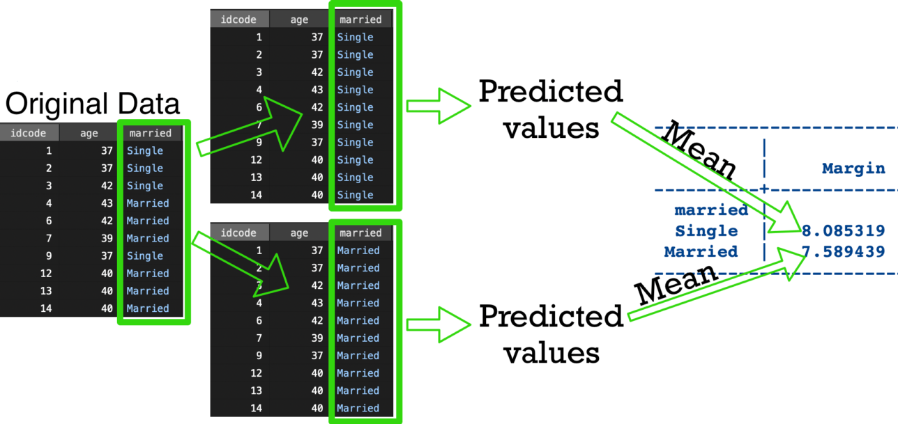
Sometimes called “as observed”.

Choices for ways to handle other covariates

As observed (default)
- Average of predicted outcomes
atmeans
- Predicted outcome at average
at specific values
- Predicted outcome at specific values
over groups
- Average of predicted outcomes only within each group
Combination (if multiple covariates)

Visualization of `margins, atmeans`

margins married, atmeans

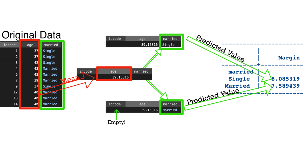
`atmeans`

. margins married, atmeans

Adjusted predictions                                     Number of obs = 2,246
Model VCE: OLS

Expression: Linear prediction, predict()
At: 0.married = .3579697 (mean)
    1.married = .6420303 (mean)
    age       = 39.15316 (mean)

------------------------------------------------------------------------------
             |            Delta-method
             |     Margin   std. err.      t    P>|t|     [95% conf. interval]
-------------+----------------------------------------------------------------
     married |
     Single  |   8.085319   .2027826    39.87   0.000     7.687658    8.482981
    Married  |   7.589439    .151412    50.12   0.000     7.292517    7.886361
------------------------------------------------------------------------------

Means for married are ignored since we’re requesting at specific values of married.
As observed and atmeans are identical for linear models; but differ for generalized linear models (we’ll see later).

`at` specific values

We can manually fix the values of other variables in the model.

margins, at(<variable> = (<numlist>) <variable2> = (<numlist>))

where <numlist> can be any of:

space-separated list of values (3 4 .5 -100)
integers between range (2/5 is equivalent to 2 3 4 5)
range with step-by instruction (3(.5)5 is equivalent to 3 3.5 4 4.5 5)
any combination of the above (3 5/7 8(.25)9)

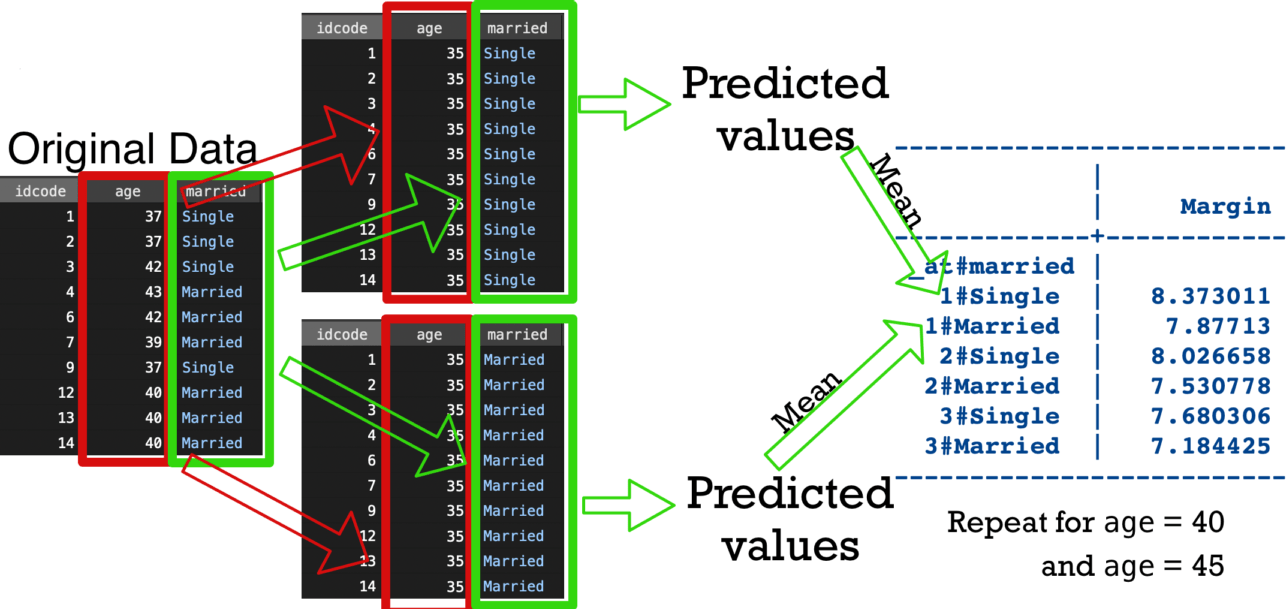
`at` specific values example

. margins married, at(age = (35(5)45))

Adjusted predictions                                     Number of obs = 2,246
Model VCE: OLS

Expression: Linear prediction, predict()
1._at: age = 35
2._at: age = 40
3._at: age = 45

------------------------------------------------------------------------------
             |            Delta-method
             |     Margin   std. err.      t    P>|t|     [95% conf. interval]
-------------+----------------------------------------------------------------
 _at#married |
   1#Single  |   8.373011   .2628879    31.85   0.000     7.857482     8.88854
  1#Married  |    7.87713   .2226589    35.38   0.000     7.440491     8.31377
   2#Single  |   8.026658   .2051185    39.13   0.000     7.624416      8.4289
  2#Married  |   7.530778   .1554066    48.46   0.000     7.226022    7.835534
   3#Single  |   7.680306   .3060744    25.09   0.000     7.080087    8.280524
  3#Married  |   7.184425   .2781542    25.83   0.000     6.638959    7.729892
------------------------------------------------------------------------------

Visualization of `margins, at(...)`

margins married, at(age = (35(5)45))

`at` without categorical variables

We can also use at with continuous variables without a categorical variable.

. margins, at(age = (35(5)45))

Predictive margins                                       Number of obs = 2,246
Model VCE: OLS

Expression: Linear prediction, predict()
1._at: age = 35
2._at: age = 40
3._at: age = 45

------------------------------------------------------------------------------
             |            Delta-method
             |     Margin   std. err.      t    P>|t|     [95% conf. interval]
-------------+----------------------------------------------------------------
         _at |
          1  |   8.054641   .2045676    39.37   0.000     7.653479    8.455802
          2  |   7.708288    .125879    61.24   0.000     7.461436     7.95514
          3  |   7.361935   .2617012    28.13   0.000     6.848734    7.875137
------------------------------------------------------------------------------

In this case, married is treated just like age was in the previous “as observed” example - held constant.

Visualization of `margins, over(...)`

margins, over(married)

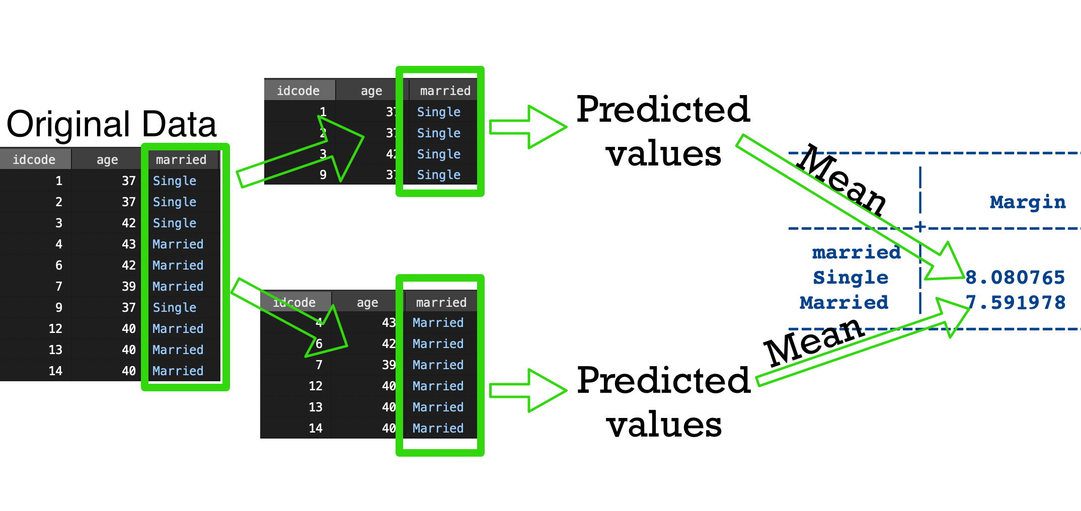
`over`

. margins, over(married)

Predictive margins                                       Number of obs = 2,246
Model VCE: OLS

Expression: Linear prediction, predict()
Over:       married

------------------------------------------------------------------------------
             |            Delta-method
             |     Margin   std. err.      t    P>|t|     [95% conf. interval]
-------------+----------------------------------------------------------------
     married |
     Single  |   8.080765   .2027658    39.85   0.000     7.683137    8.478394
    Married  |   7.591978    .151405    50.14   0.000     7.295069    7.888887
------------------------------------------------------------------------------

Combining some of these effects

We can combine some of these when we have multiple predictors. For example,

. regress wage age i.married i.south, noheader
------------------------------------------------------------------------------
        wage | Coefficient  Std. err.      t    P>|t|     [95% conf. interval]
-------------+----------------------------------------------------------------
         age |  -.0675817   .0393325    -1.72   0.086    -.1447135    .0095502
             |
     married |
    Married  |  -.5039005   .2509983    -2.01   0.045    -.9961138   -.0116873
             |
       south |
      South  |  -1.514432   .2438214    -6.21   0.000    -1.992572   -1.036293
       _cons |   11.37168   1.558336     7.30   0.000     8.315744    14.42761
------------------------------------------------------------------------------

Combining some of these effects, 2

regress wage age i.married i.south

. margins married, at(south = (1)) atmeans

Adjusted predictions                                     Number of obs = 2,246
Model VCE: OLS

Expression: Linear prediction, predict()
At: age       = 39.15316 (mean)
    0.married = .3579697 (mean)
    1.married = .6420303 (mean)
    south     =        1

------------------------------------------------------------------------------
             |            Delta-method
             |     Margin   std. err.      t    P>|t|     [95% conf. interval]
-------------+----------------------------------------------------------------
     married |
     Single  |   7.211208   .2454553    29.38   0.000     6.729864    7.692551
    Married  |   6.707307   .2066834    32.45   0.000     6.301996    7.112618
------------------------------------------------------------------------------

Note the use of a categorical variable (south) in at().
Recall that married’s means are ignored.

Estimated slopes

Everything we’ve done so far is estimating means. We can estimate slopes with the dydx option.

. regress wage age, noheader
------------------------------------------------------------------------------
        wage | Coefficient  Std. err.      t    P>|t|     [95% conf. interval]
-------------+----------------------------------------------------------------
         age |  -.0680236   .0396796    -1.71   0.087    -.1458362     .009789
       _cons |   10.43029   1.558318     6.69   0.000     7.374394    13.48618
------------------------------------------------------------------------------

. margins, dydx(age)

Average marginal effects                                 Number of obs = 2,246
Model VCE: OLS

Expression: Linear prediction, predict()
dy/dx wrt:  age

------------------------------------------------------------------------------
             |            Delta-method
             |      dy/dx   std. err.      t    P>|t|     [95% conf. interval]
-------------+----------------------------------------------------------------
         age |  -.0680236   .0396796    -1.71   0.087    -.1458362     .009789
------------------------------------------------------------------------------

Non-linear relationships

. regress wage c.age##c.age, noheader
------------------------------------------------------------------------------
        wage | Coefficient  Std. err.      t    P>|t|     [95% conf. interval]
-------------+----------------------------------------------------------------
         age |   .7033681   1.084471     0.65   0.517    -1.423304     2.83004
             |
 c.age#c.age |  -.0097745   .0137323    -0.71   0.477    -.0367039     .017155
             |
       _cons |  -4.696709   21.30931    -0.22   0.826    -46.48474    37.09133
------------------------------------------------------------------------------

. margins, dydx(age)

Average marginal effects                                 Number of obs = 2,246
Model VCE: OLS

Expression: Linear prediction, predict()
dy/dx wrt:  age

------------------------------------------------------------------------------
             |            Delta-method
             |      dy/dx   std. err.      t    P>|t|     [95% conf. interval]
-------------+----------------------------------------------------------------
         age |  -.0620333   .0405666    -1.53   0.126    -.1415852    .0175186
------------------------------------------------------------------------------

Estimated marginal slopes, comments

This will get a lot more useful when we discuss interactions next.
Handling additional covariates with “as observed”/atmeans or at continues to work.
In linear models, “average slope” and “slope at average” are equivalent - not true in non-linear models.
There are additional options such as eyex for “elasticities”, an extremely similar concept in econometrics.

Instantaneous slopes

For non-linear trends, the slope changes across values of the predictor.

(This is also the tangent, and is obtained by taking the derivative, which is often written as \(\frac{dy}{dx}\), hence the option dydx.)

Estimating the instantaneous slope

regress wage c.age##c.age

. margins, dydx(age) at(age = (35 40 45))

Conditional marginal effects                             Number of obs = 2,246
Model VCE: OLS

Expression: Linear prediction, predict()
dy/dx wrt:  age
1._at: age = 35
2._at: age = 40
3._at: age = 45

------------------------------------------------------------------------------
             |            Delta-method
             |      dy/dx   std. err.      t    P>|t|     [95% conf. interval]
-------------+----------------------------------------------------------------
age          |
         _at |
          1  |   .0191564   .1287496     0.15   0.882    -.2333243    .2716372
          2  |  -.0785881   .0423687    -1.85   0.064    -.1616741     .004498
          3  |  -.1763326   .1572552    -1.12   0.262    -.4847135    .1320483
------------------------------------------------------------------------------

Examining interactions

Recall our starting example with a categorical variable and the regression coefficients only telling part of the story.

regress wage i.race

Group	Average	Comparison	Estimate
White	8.083	Black vs White	-1.238
Black	???	Other vs White	0.468
Other	???	Other vs Black	???

We only get 50% of relevant pieces of information from the regression coefficients.

When we begin to include interactions in the model, even less useful information can be extracted via regression coefficients alone.

Categorical-categorical interaction

. regress wage i.married##i.race, noheader
------------------------------------------------------------------------------
        wage | Coefficient  Std. err.      t    P>|t|     [95% conf. interval]
-------------+----------------------------------------------------------------
     married |
    Married  |  -1.204674    .309034    -3.90   0.000    -1.810697   -.5986511
             |
        race |
      Black  |  -2.194947    .415727    -5.28   0.000    -3.010198   -1.379697
      Other  |  -.4967496   2.037457    -0.24   0.807    -4.492251    3.498752
             |
married#race |
    Married #|
      Black  |   1.439186   .5661142     2.54   0.011     .3290224    2.549349
    Married #|
      Other  |   1.375469   2.448432     0.56   0.574    -3.425963    6.176901
             |
       _cons |   8.929288   .2590186    34.47   0.000     8.421347     9.43723
------------------------------------------------------------------------------

\(3\times2 = 6\) averages, \(\binom{6}{2} = 15\) pairwise differences in averages.

Regression coefficients: 1 estimated average, 5 estimated pairwise differences - only 29% of relevant pieces of information!

`margins` syntax with interactions

Average of each level of married, averaged across race:
```
margins married
```
Average of each unique subgroup of married and race:
```
margins married#race
```
Note the single # instead of the ## in the model. Putting ## would produce all of margins married, margins race, and margins married#race.

Pairwise differences between all unique subgroups:

margins married#race, pwcompare(ci) // default
margins married#race, pwcompare(pv)

Average effect of marriage within levels of race:
```
margins married@race, contrast(ci nowald)
margins married@race, contrast(pv nowald)
```
Note the use of @ instead of # when dealing with the contrast() option.

Marginal effects

. margins married

Predictive margins                                       Number of obs = 2,246
Model VCE: OLS

Expression: Linear prediction, predict()

------------------------------------------------------------------------------
             |            Delta-method
             |     Margin   std. err.      t    P>|t|     [95% conf. interval]
-------------+----------------------------------------------------------------
     married |
     Single  |    8.35379   .2081151    40.14   0.000     7.945671    8.761909
    Married  |   7.538612   .1528743    49.31   0.000     7.238821    7.838402
------------------------------------------------------------------------------

Estimated means in all unique subgroups

. margins married#race

Adjusted predictions                                     Number of obs = 2,246
Model VCE: OLS

Expression: Linear prediction, predict()

------------------------------------------------------------------------------
             |            Delta-method
             |     Margin   std. err.      t    P>|t|     [95% conf. interval]
-------------+----------------------------------------------------------------
married#race |
     Single #|
      White  |   8.929288   .2590186    34.47   0.000     8.421347     9.43723
     Single #|
      Black  |   6.734341   .3251742    20.71   0.000     6.096667    7.372016
     Single #|
      Other  |   8.432539   2.020926     4.17   0.000     4.469456    12.39562
    Married #|
      White  |   7.724614   .1685569    45.83   0.000      7.39407    8.055158
    Married #|
      Black  |   6.968853   .3453187    20.18   0.000     6.291675    7.646031
    Married #|
      Other  |   8.603333   1.347284     6.39   0.000     5.961278    11.24539
------------------------------------------------------------------------------

All pairwise comparisons

. margins married#race, pwcompare(pv)

Pairwise comparisons of adjusted predictions             Number of obs = 2,246
Model VCE: OLS

Expression: Linear prediction, predict()

----------------------------------------------------------------------------
                                    |            Delta-method    Unadjusted
                                    |   Contrast   std. err.      t    P>|t|
------------------------------------+---------------------------------------
                       married#race |
  (Single#Black) vs (Single#White)  |  -2.194947    .415727    -5.28   0.000
  (Single#Other) vs (Single#White)  |  -.4967496   2.037457    -0.24   0.807
 (Married#White) vs (Single#White)  |  -1.204674    .309034    -3.90   0.000
 (Married#Black) vs (Single#White)  |  -1.960435   .4316661    -4.54   0.000
 (Married#Other) vs (Single#White)  |  -.3259551   1.371956    -0.24   0.812
  (Single#Other) vs (Single#Black)  |   1.698198    2.04692     0.83   0.407
 (Married#White) vs (Single#Black)  |   .9902731   .3662645     2.70   0.007
 (Married#Black) vs (Single#Black)  |   .2345117    .474324     0.49   0.621
 (Married#Other) vs (Single#Black)  |   1.868992    1.38597     1.35   0.178
 (Married#White) vs (Single#Other)  |  -.7079245   2.027943    -0.35   0.727
 (Married#Black) vs (Single#Other)  |  -1.463686   2.050216    -0.71   0.475
 (Married#Other) vs (Single#Other)  |   .1707945   2.428851     0.07   0.944
(Married#Black) vs (Married#White)  |  -.7557614   .3842609    -1.97   0.049
(Married#Other) vs (Married#White)  |    .878719   1.357787     0.65   0.518
(Married#Other) vs (Married#Black)  |    1.63448   1.390834     1.18   0.240
----------------------------------------------------------------------------

Effect of `married` within each `race`

. margins married@race, contrast(pv nowald)

Contrasts of adjusted predictions                        Number of obs = 2,246
Model VCE: OLS

Expression: Linear prediction, predict()

-----------------------------------------------------------------
                         |            Delta-method
                         |   Contrast   std. err.      t    P>|t|
-------------------------+---------------------------------------
            married@race |
(Married vs base) White  |  -1.204674    .309034    -3.90   0.000
(Married vs base) Black  |   .2345117    .474324     0.49   0.621
(Married vs base) Other  |   .1707945   2.428851     0.07   0.944
-----------------------------------------------------------------

Note the use of @ again.

`contrast` options

We can run just margins married@race without a contrast argument but it will only produce a Wald test table. Switching married@race to race@married:

. margins race@married

Contrasts of adjusted predictions                        Number of obs = 2,246
Model VCE: OLS

Expression: Linear prediction, predict()

------------------------------------------------
             |         df           F        P>F
-------------+----------------------------------
race@married |
     Single  |          2       13.95     0.0000
    Married  |          2        2.22     0.1089
      Joint  |          4        8.09     0.0000
             |
 Denominator |       2240
------------------------------------------------

nowald option to contrast suppresses this table; pv or ci produce the estimate table. (So contrast(ci) without nowald would produce both tables.)

Effect of `race` within each `married`

. margins race@married, contrast(pv nowald)

Contrasts of adjusted predictions                        Number of obs = 2,246
Model VCE: OLS

Expression: Linear prediction, predict()

-----------------------------------------------------------------
                         |            Delta-method
                         |   Contrast   std. err.      t    P>|t|
-------------------------+---------------------------------------
            race@married |
 (Black vs base) Single  |  -2.194947    .415727    -5.28   0.000
(Black vs base) Married  |  -.7557614   .3842609    -1.97   0.049
 (Other vs base) Single  |  -.4967496   2.037457    -0.24   0.807
(Other vs base) Married  |    .878719   1.357787     0.65   0.518
-----------------------------------------------------------------

Since race has more than 2 categories, each comparison is against a reference category. This isn’t a problem if the first variable in the margins call is binary, but is annoying otherwise.

Displaying all pairwise comparisons within `married` status

. margins race, at(married = (0)) pwcompare(pv)

Pairwise comparisons of adjusted predictions             Number of obs = 2,246
Model VCE: OLS

Expression: Linear prediction, predict()
At: married = 0

--------------------------------------------------------
                |            Delta-method    Unadjusted
                |   Contrast   std. err.      t    P>|t|
----------------+---------------------------------------
           race |
Black vs White  |  -2.194947    .415727    -5.28   0.000
Other vs White  |  -.4967496   2.037457    -0.24   0.807
Other vs Black  |   1.698198    2.04692     0.83   0.407
--------------------------------------------------------

Repeat for married = (1)

Categorical-continuous interactions

. regress wage c.age##i.race, noheader
------------------------------------------------------------------------------
        wage | Coefficient  Std. err.      t    P>|t|     [95% conf. interval]
-------------+----------------------------------------------------------------
         age |  -.0545975   .0459913    -1.19   0.235    -.1447876    .0355926
             |
        race |
      Black  |   1.403328   3.590285     0.39   0.696    -5.637306    8.443963
      Other  |   27.42823   14.02561     1.96   0.051    -.0763282    54.93278
             |
  race#c.age |
      Black  |  -.0687157   .0919576    -0.75   0.455    -.2490468    .1116154
      Other  |  -.6858332   .3556579    -1.93   0.054    -1.383287    .0116202
             |
       _cons |   10.22718   1.811727     5.64   0.000     6.674339    13.78002
------------------------------------------------------------------------------

Group	Slope
White	-0.055
Black	???
Other	???

Comparison	Diff. in slopes
Black vs White	-0.069
Other vs White	-0.686
Other vs Black	???

Estimating marginal slopes in each `race`

. margins race, dydx(age)

Average marginal effects                                 Number of obs = 2,246
Model VCE: OLS

Expression: Linear prediction, predict()
dy/dx wrt:  age

------------------------------------------------------------------------------
             |            Delta-method
             |      dy/dx   std. err.      t    P>|t|     [95% conf. interval]
-------------+----------------------------------------------------------------
age          |
        race |
      White  |  -.0545975   .0459913    -1.19   0.235    -.1447876    .0355926
      Black  |  -.1233132   .0796304    -1.55   0.122    -.2794703    .0328439
      Other  |  -.7404307   .3526717    -2.10   0.036    -1.432028   -.0488332
------------------------------------------------------------------------------

Testing for differences between marginal slopes

. margins race, dydx(age) pwcompare(pv)

Pairwise comparisons of average marginal effects

Model VCE: OLS                                           Number of obs = 2,246

Expression: Linear prediction, predict()
dy/dx wrt:  age

--------------------------------------------------------
                |   Contrast Delta-method    Unadjusted
                |      dy/dx   std. err.      t    P>|t|
----------------+---------------------------------------
age             |
           race |
Black vs White  |  -.0687157   .0919576    -0.75   0.455
Other vs White  |  -.6858332   .3556579    -1.93   0.054
Other vs Black  |  -.6171175   .3615499    -1.71   0.088
--------------------------------------------------------

Looking at it the other way

Prior was “Differences in effect of age across race”. Now looking at “differences in races across values of age”:

. margins race, at(age = (35 45))

Adjusted predictions                                     Number of obs = 2,246
Model VCE: OLS

Expression: Linear prediction, predict()
1._at: age = 35
2._at: age = 45

------------------------------------------------------------------------------
             |            Delta-method
             |     Margin   std. err.      t    P>|t|     [95% conf. interval]
-------------+----------------------------------------------------------------
    _at#race |
    1#White  |   8.316265   .2421443    34.34   0.000     7.841414    8.791115
    1#Black  |   7.314544   .3851413    18.99   0.000     6.559273    8.069815
    1#Other  |   11.74033   1.889093     6.21   0.000     8.035773    15.44488
    2#White  |   7.770289   .2990187    25.99   0.000     7.183907    8.356672
    2#Black  |   6.081412   .5468841    11.12   0.000     5.008959    7.153865
    2#Other  |   4.336022   2.300178     1.89   0.060    -.1746818    8.846725
------------------------------------------------------------------------------

Testing for differences of marginal means at specific values of `age`

. margins race, at(age = (35)) pwcompare(pv)

Pairwise comparisons of adjusted predictions             Number of obs = 2,246
Model VCE: OLS

Expression: Linear prediction, predict()
At: age = 35

--------------------------------------------------------
                |            Delta-method    Unadjusted
                |   Contrast   std. err.      t    P>|t|
----------------+---------------------------------------
           race |
Black vs White  |  -1.001721    .454937    -2.20   0.028
Other vs White  |   3.424064   1.904549     1.80   0.072
Other vs Black  |   4.425785   1.927954     2.30   0.022
--------------------------------------------------------

If our at contains multiple values of age, we’ll get too many uninteresting results, so repeat with margins race, at(age = (45)) pwcompare(pv).

Be precise your choice of age values - junk in, junk out.

Continuous-continuous interactions

With a continuous-continuous interaction, we generally want to estimate the slope of one variable at specific values of the other variable.

. regress wage c.age##c.ttl_exp

      Source |       SS           df       MS      Number of obs   =     2,246
-------------+----------------------------------   F(3, 2242)      =     62.17
       Model |  5711.33802         3  1903.77934   Prob > F        =    0.0000
    Residual |  68656.6294     2,242  30.6229391   R-squared       =    0.0768
-------------+----------------------------------   Adj R-squared   =    0.0756
       Total |  74367.9674     2,245  33.1260434   Root MSE        =    5.5338

------------------------------------------------------------------------------
        wage | Coefficient  Std. err.      t    P>|t|     [95% conf. interval]
-------------+----------------------------------------------------------------
         age |   .0585611   .1082827     0.54   0.589    -.1537837    .2709059
     ttl_exp |   .9585974   .3281056     2.92   0.004     .3151748     1.60202
             |
       c.age#|
   c.ttl_exp |  -.0155082   .0082317    -1.88   0.060    -.0316508    .0006343
             |
       _cons |   1.096482   4.282121     0.26   0.798    -7.300854    9.493817
------------------------------------------------------------------------------

Marginal slope at specific values

. margins, dydx(age) at(ttl_exp = (5(5)20))

Average marginal effects                                 Number of obs = 2,246
Model VCE: OLS

Expression: Linear prediction, predict()
dy/dx wrt:  age
1._at: ttl_exp =  5
2._at: ttl_exp = 10
3._at: ttl_exp = 15
4._at: ttl_exp = 20

------------------------------------------------------------------------------
             |            Delta-method
             |      dy/dx   std. err.      t    P>|t|     [95% conf. interval]
-------------+----------------------------------------------------------------
age          |
         _at |
          1  |  -.0189801   .0713234    -0.27   0.790    -.1588469    .1208867
          2  |  -.0965213   .0428597    -2.25   0.024    -.1805701   -.0124725
          3  |  -.1740626     .04444    -3.92   0.000    -.2612104   -.0869147
          4  |  -.2516038   .0741681    -3.39   0.001    -.3970492   -.1061584
------------------------------------------------------------------------------

We can of course reverse the “focal” variable with the “moderator”: margins, dydx(ttl_exp) at(age = (35(5)45)).

Choosing values of continuous variables

Be sure to choose reasonable values of continuous variables.

. hist ttl_exp
(bin=33, start=.11538462, width=.87179486)

`marginsplot`

marginsplot is a post-post-estimation command
- You can run it after a margins call.
Any margins call with pairwise comparisons (pwcompare or using @) may produce silly results.
marginsplot takes a lot of the standard plotting options. There are a few specific options that are useful:
- xdim() defines the x-axis, useful if Stata chooses the wrong by default
- recast() allows us to use a different plot type for the estimates.
- recastci() allows us to use a different plot type for the confidence bounds.
marginsplot when there’s an interaction produces an “interaction plot.”

Estimated means

. quietly regress wage i.race

. quietly margins race

. marginsplot

Variables that uniquely identify margins: race

Estimated means as bar chart

. marginsplot, recast(bar)

Variables that uniquely identify margins: race

Plotting non-linear slopes

. quietly regress wage c.age##c.age

. margins, dydx(age) at(age = (35(5)45))

Conditional marginal effects                             Number of obs = 2,246
Model VCE: OLS

Expression: Linear prediction, predict()
dy/dx wrt:  age
1._at: age = 35
2._at: age = 40
3._at: age = 45

------------------------------------------------------------------------------
             |            Delta-method
             |      dy/dx   std. err.      t    P>|t|     [95% conf. interval]
-------------+----------------------------------------------------------------
age          |
         _at |
          1  |   .0191564   .1287496     0.15   0.882    -.2333243    .2716372
          2  |  -.0785881   .0423687    -1.85   0.064    -.1616741     .004498
          3  |  -.1763326   .1572552    -1.12   0.262    -.4847135    .1320483
------------------------------------------------------------------------------

Plotting non-linear slopes, 2

. quietly margins, at(age = (35(.5)45)) nose

. marginsplot, recast(line)

Variables that uniquely identify margins: age

nose option suppresses standard errors and performs much faster calculation too! I don’t recommend this for final results, but useful during development of models.

Interaction plot, categorical-continuous

. quietly regress wage i.race##c.age

. quietly margins race, at(age = (35(5)45))

. marginsplot

Variables that uniquely identify margins: age race

Interaction plot, continuous-continuous

. quietly regress wage c.ttl_exp##c.age

. quietly margins, at(age = (35(5)45) ttl_exp = (5(5)15))

. marginsplot

Variables that uniquely identify margins: age ttl_exp

Switching the x-dimension

. quietly regress wage c.ttl_exp##c.age

. quietly margins, at(age = (35(5)45) ttl_exp = (5(5)15))

. marginsplot, xdim(ttl_exp)

Variables that uniquely identify margins: age ttl_exp

`margins` with non-linear models

The margins command produces estimates on the scale of the outcome. E.g. for a logistic regression model, the results are in the probability scale.

. logit union c.hours##i.married, or nolog

Logistic regression                                     Number of obs =  1,877
                                                        LR chi2(3)    =  12.03
                                                        Prob > chi2   = 0.0073
Log likelihood = -1040.3272                             Pseudo R2     = 0.0057

------------------------------------------------------------------------------
       union | Odds ratio   Std. err.      z    P>|z|     [95% conf. interval]
-------------+----------------------------------------------------------------
       hours |   1.001253   .0108298     0.12   0.908     .9802502    1.022705
             |
     married |
    Married  |   .4305923   .2201786    -1.65   0.099      .158057    1.173056
             |
     married#|
     c.hours |
    Married  |    1.01625   .0129394     1.27   0.206     .9912034     1.04193
             |
       _cons |   .3632802   .1597701    -2.30   0.021      .153421    .8601988
------------------------------------------------------------------------------
Note: _cons estimates baseline odds.

`margins` after `logit`

. margins married, at(hours = 40)

Adjusted predictions                                     Number of obs = 1,877
Model VCE: OIM

Expression: Pr(union), predict()
At: hours = 40

------------------------------------------------------------------------------
             |            Delta-method
             |     Margin   std. err.      z    P>|z|     [95% conf. interval]
-------------+----------------------------------------------------------------
     married |
     Single  |   .2763779   .0174778    15.81   0.000     .2421221    .3106337
    Married  |   .2386115   .0127765    18.68   0.000       .21357    .2636531
------------------------------------------------------------------------------

Thus the model predicts that 27.64% of unmarried workers and 23.86% of married workers have a positive outcome when working 40 hour weeks.

“as observed” vs `atmeans`

. margins married

Predictive margins                                       Number of obs = 1,877
Model VCE: OIM

Expression: Pr(union), predict()

------------------------------------------------------------------------------
             |            Delta-method
             |     Margin   std. err.      z    P>|z|     [95% conf. interval]
-------------+----------------------------------------------------------------
     married |
     Single  |   .2757857   .0180805    15.25   0.000     .2403486    .3112228
    Married  |   .2325589    .012185    19.09   0.000     .2086768    .2564411
------------------------------------------------------------------------------

. margins married, atmeans

Adjusted predictions                                     Number of obs = 1,877
Model VCE: OIM

Expression: Pr(union), predict()
At: hours     = 37.60522 (mean)
    0.married = .3489611 (mean)
    1.married = .6510389 (mean)

------------------------------------------------------------------------------
             |            Delta-method
             |     Margin   std. err.      z    P>|z|     [95% conf. interval]
-------------+----------------------------------------------------------------
     married |
     Single  |   .2757787   .0181128    15.23   0.000     .2402783    .3112791
    Married  |   .2311359   .0121309    19.05   0.000     .2073598     .254912
------------------------------------------------------------------------------

`marginsplot` after `logit`

. quietly margins married, at(hours = (30 40 50))

. marginsplot, recastci(rarea) ciopt(color(%20))

Variables that uniquely identify margins: hours married

Count models

For Poisson models (or negative binomial), the results are in the count scale.

. poisson wage i.married##c.hours
note: noncount dependent variable encountered; if you are fitting an
      exponential-mean model, consider using robust standard errors.

Iteration 0:  Log likelihood = -7536.5998  
Iteration 1:  Log likelihood = -7536.5998  

Poisson regression                                      Number of obs =  2,242
                                                        LR chi2(3)    = 262.83
                                                        Prob > chi2   = 0.0000
Log likelihood = -7536.5998                             Pseudo R2     = 0.0171

------------------------------------------------------------------------------
        wage | Coefficient  Std. err.      z    P>|z|     [95% conf. interval]
-------------+----------------------------------------------------------------
     married |
    Married  |   .1773426   .0672074     2.64   0.008     .0456186    .3090667
       hours |   .0152061   .0013874    10.96   0.000     .0124868    .0179255
             |
     married#|
     c.hours |
    Married  |    -.00528   .0016525    -3.20   0.001    -.0085188   -.0020411
             |
       _cons |   1.485806   .0575035    25.84   0.000     1.373101     1.59851
------------------------------------------------------------------------------

`margins` after `poisson`

. margins married, at(hours = 40)

Adjusted predictions                                     Number of obs = 2,242
Model VCE: OIM

Expression: Predicted number of events, predict()
At: hours = 40

------------------------------------------------------------------------------
             |            Delta-method
             |     Margin   std. err.      z    P>|z|     [95% conf. interval]
-------------+----------------------------------------------------------------
     married |
     Single  |   8.117728   .1009178    80.44   0.000     7.919933    8.315523
    Married  |   7.847492   .0774572   101.31   0.000     7.695679    7.999306
------------------------------------------------------------------------------

`marginsplot` after `poisson`

. quietly margins married, at(hours = (35 40 45))

. marginsplot, yscale(range(6 10)) ylabel(6(1)10)

Variables that uniquely identify margins: hours married

`margins` versus regression coefficients

Of course, in GLMs, the estimated coefficients are not additive on the scale of the outcome.

logistic models: odds ratios
count models: incidence rate ratios

However, margins does produce results on the outcome scale.

Therefore, margins is not an appropriate tool to, for example, obtain odds ratios between all pairs of groups in a categorical variable.

So why use `margins` after a non-linear model?

Probabilities and counts are easily to interpret than odds ratios and rate ratios.
Interaction plots are easier to interpret that regression coefficients.

If you do want odds ratios…

..use the nlcom post-estimation command:

. logit union i.race, nolog or

Logistic regression                                     Number of obs =  1,878
                                                        LR chi2(2)    =  12.71
                                                        Prob > chi2   = 0.0017
Log likelihood = -1040.2692                             Pseudo R2     = 0.0061

------------------------------------------------------------------------------
       union | Odds ratio   Std. err.      z    P>|z|     [95% conf. interval]
-------------+----------------------------------------------------------------
        race |
      Black  |   1.501429   .1760094     3.47   0.001     1.193219    1.889249
      Other  |   1.740066   .7619876     1.26   0.206     .7375959    4.104999
             |
       _cons |   .2873454   .0187607   -19.10   0.000     .2528306    .3265719
------------------------------------------------------------------------------
Note: _cons estimates baseline odds.

. logit, coeflegend

Logistic regression                                     Number of obs =  1,878
                                                        LR chi2(2)    =  12.71
                                                        Prob > chi2   = 0.0017
Log likelihood = -1040.2692                             Pseudo R2     = 0.0061

------------------------------------------------------------------------------
       union | Coefficient  Legend
-------------+----------------------------------------------------------------
        race |
      Black  |    .406417  _b[2.race]
      Other  |   .5539232  _b[3.race]
             |
       _cons |   -1.24707  _b[_cons]
------------------------------------------------------------------------------

. nlcom (black_white: exp(_b[2.race])) (other_white: exp(_b[3.race])) ///
>     (other_black: exp(_b[2.race] - _b[3.race]))

 black_white: exp(_b[2.race])
 other_white: exp(_b[3.race])
 other_black: exp(_b[2.race] - _b[3.race])

------------------------------------------------------------------------------
       union | Coefficient  Std. err.      z    P>|z|     [95% conf. interval]
-------------+----------------------------------------------------------------
 black_white |   1.501429   .1760094     8.53   0.000     1.156456    1.846401
 other_white |   1.740066   .7619876     2.28   0.022     .2465981    3.233534
 other_black |   .8628571   .3829566     2.25   0.024     .1122759    1.613438
------------------------------------------------------------------------------

Miscellaneous things about `margins`

margins are not fitting a different model! It is not a separate model or analysis.
Higher-order interactions work as expected:
- regress y a##b##c
- margins a#b#c (if all categorical)
- margin a#c, at(b = (3 5))
The expression option can apply transformations to margins.
- E.g. after logit to get things on probability scale:
  - margins, expression(100*predict(pr))
post option turns margins into an estimation command

Other resources

https://errickson.net/marginsnotes/
- Worked examples of a number of different marginal targets, including code for both Stata and R
https://www.stata.com/manuals/rmargins.pdf
- 58 pages
https://www.stata.com/manuals/rmarginsplot.pdf
- 35 pages

Stata’s margins command

Post-estimation command

Categorical variables

Fitting the model

Calculating group effects and comparisons

Changing reference category

Estimated means

Differences in estimated means

Syntax for estimated means

In the presence of covariates

Visualization of margins

Choices for ways to handle other covariates

Visualization of margins, atmeans

atmeans

at specific values

at specific values example

Visualization of margins, at(...)

at without categorical variables

Visualization of margins, over(...)

over

Combining some of these effects

Combining some of these effects, 2

Estimated slopes

Non-linear relationships

Estimated marginal slopes, comments

Instantaneous slopes

Estimating the instantaneous slope

Examining interactions

Categorical-categorical interaction

margins syntax with interactions

Marginal effects

Estimated means in all unique subgroups

All pairwise comparisons

Effect of married within each race

contrast options

Effect of race within each married

Displaying all pairwise comparisons within married status

Categorical-continuous interactions

Estimating marginal slopes in each race

Testing for differences between marginal slopes

Looking at it the other way

Testing for differences of marginal means at specific values of age

Continuous-continuous interactions

Marginal slope at specific values

Choosing values of continuous variables

marginsplot

Estimated means

Estimated means as bar chart

Plotting non-linear slopes

Plotting non-linear slopes, 2

Interaction plot, categorical-continuous

Interaction plot, continuous-continuous

Switching the x-dimension

margins with non-linear models

margins after logit

“as observed” vs atmeans

marginsplot after logit

Count models

margins after poisson

marginsplot after poisson

margins versus regression coefficients

So why use margins after a non-linear model?

If you do want odds ratios…

Miscellaneous things about margins

Other resources

Stata’s `margins` command

Visualization of `margins`

Visualization of `margins, atmeans`

`atmeans`

`at` specific values

`at` specific values example

Visualization of `margins, at(...)`

`at` without categorical variables

Visualization of `margins, over(...)`

`over`

`margins` syntax with interactions

Effect of `married` within each `race`

`contrast` options

Effect of `race` within each `married`

Displaying all pairwise comparisons within `married` status

Estimating marginal slopes in each `race`

Testing for differences of marginal means at specific values of `age`

`marginsplot`

`margins` with non-linear models

`margins` after `logit`

“as observed” vs `atmeans`

`marginsplot` after `logit`

`margins` after `poisson`

`marginsplot` after `poisson`

`margins` versus regression coefficients

So why use `margins` after a non-linear model?

Miscellaneous things about `margins`