Matching with R: Strategies for Larger Data

Josh Errickson

2024-04-01

Outline

  1. Review of propensity scores and matching
  2. Separating PS and matching
  3. Introduction to optmatch
  4. Optimal and full matching
  5. Speeding up matching
  6. Final example

Review of Matching

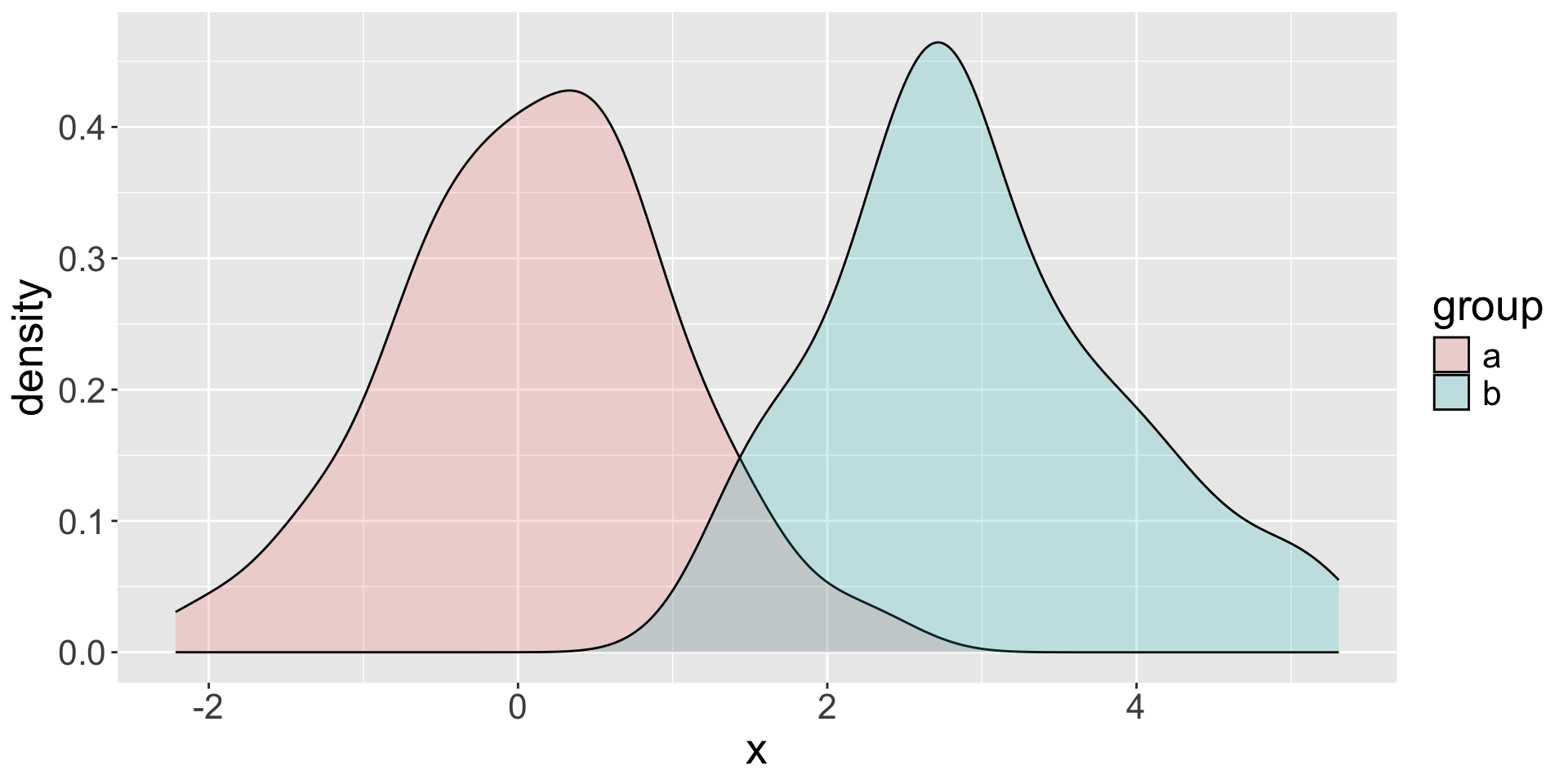
Overlap & Balance #1

  • Overlap: Are variables observed over the same range for both groups?

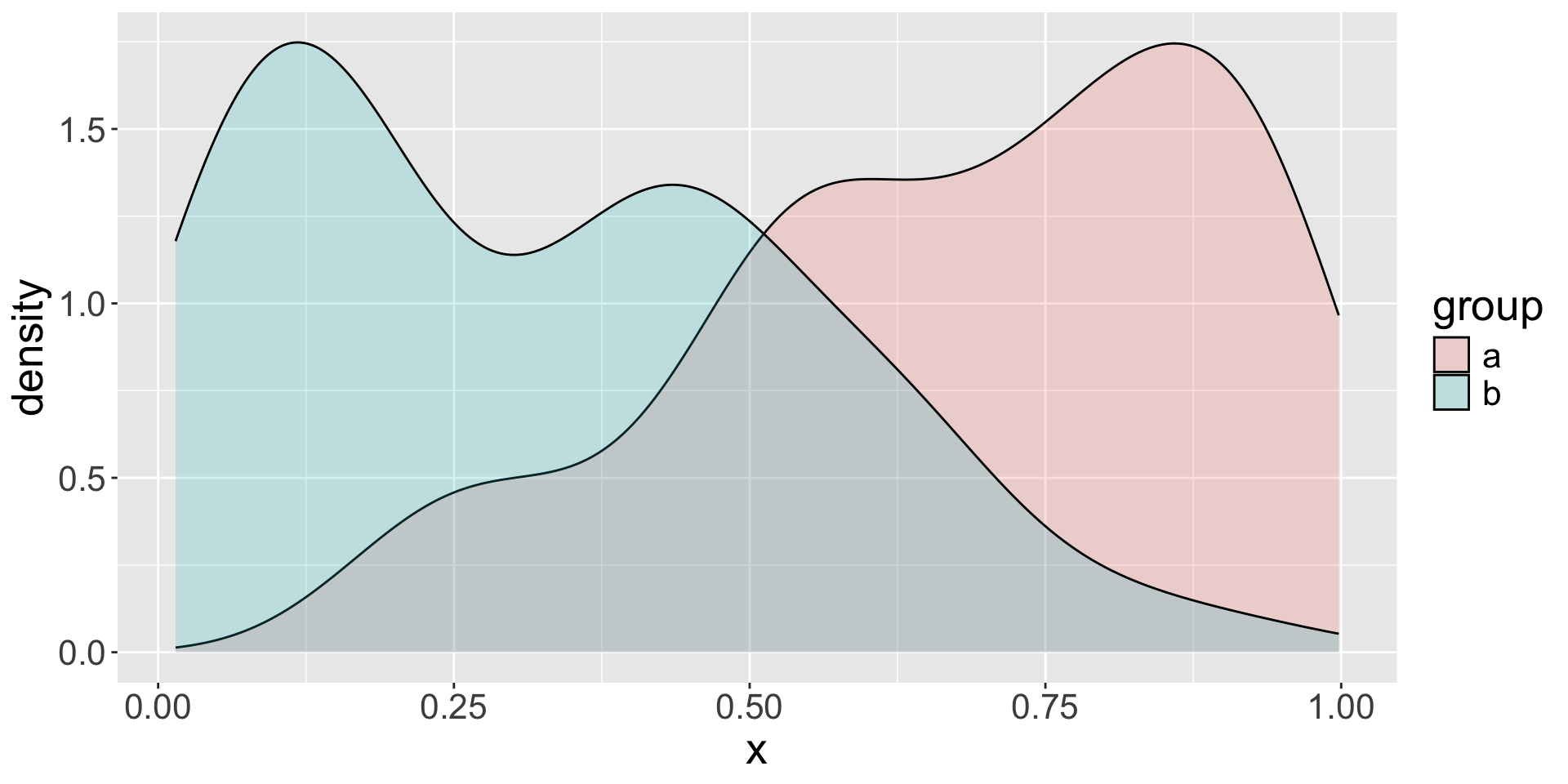
Overlap & Balance #2

  • Balance: Are the distributions of variables the same for both groups?

Overlap & Balance #3

  • Matching is very good at addressing partial overlap.
  • Propensity score matching is theoretically good at addressing imbalance.
    • Practically maybe not.
  • Weighting/Regression may be better at addressing imbalance solely.

Overlap & Balance #4

  • Overlap is easy to observe and quantify, and comes for “free” with matching, so usually not a focus.
  • Balance is moderately hard to observe and quantify (especially in higher dimensions) and will be the focus of matching

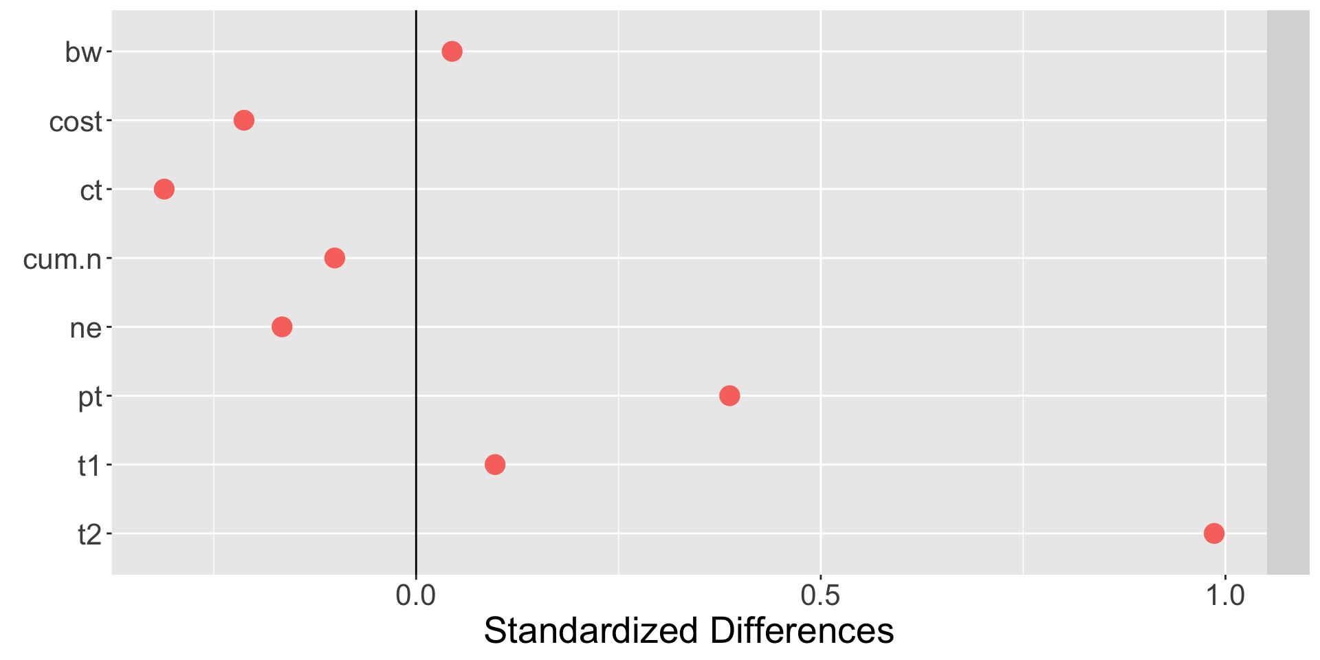
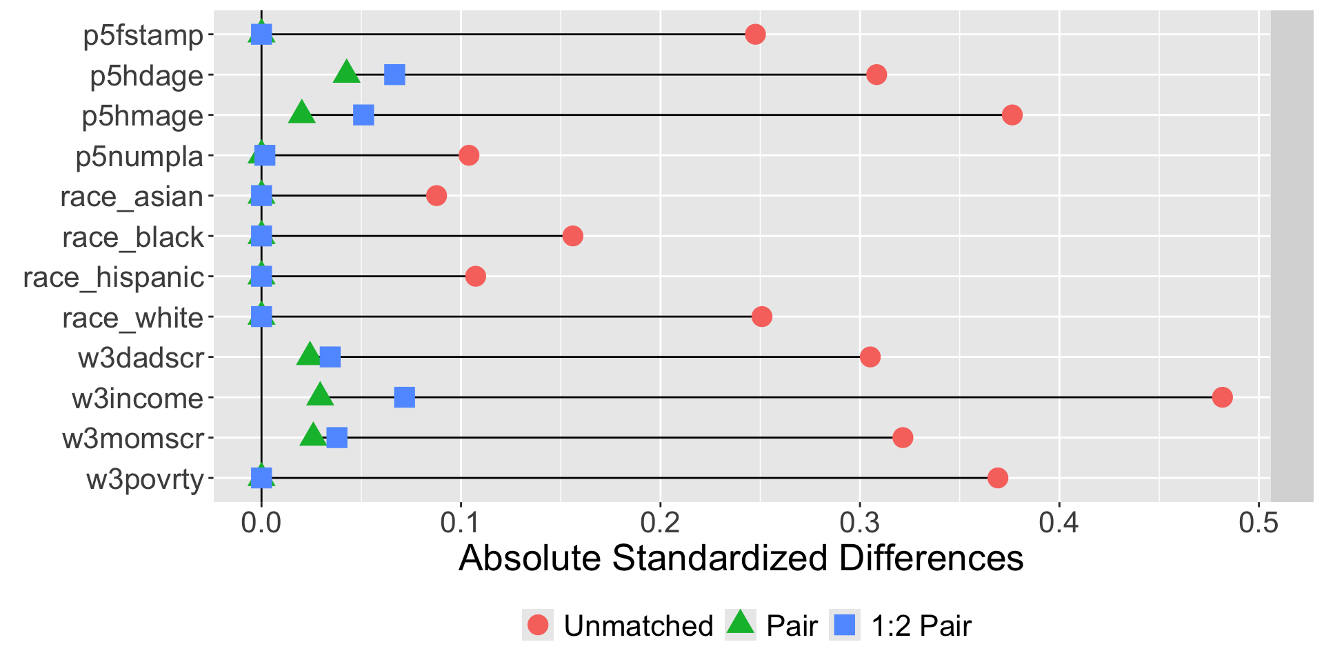
Love plot

Distance

  • How “far away” are a pair of observations?
    • Easy for 1 dimension, less clear for more dimensions.
  • Can define distance however you want
  • Common choices:
    • Euclidean
    • Mahalanobis

Measuring match quality

  • Formal goal: Balance
    • Harder to define
    • Is often multi-dimensional
  • Instead, measure total distance within a matched set
  • Goal: Minimize distance in matched sets
  • Strong correlation between balance and distance

Propensity Score Matching

  • Matching on more than one covariate is challenging.

\[ ps_i(\mathbf{X}_i) = P(Z_i = 1 | \mathbf{X}_i) \]

  • Probability of an observation being in group 1 (usually treatment) given their characteristics.
  • Propensity scores can be thought of as dimension reduction.
  • Scores are usually estimated by logistic regression predicting group membership.
    • “Kitchen sink”
    • Potentially exclude variables associated with treatment but not outcome. (Austin 2011, 414–15)

Main Benefit of PS matching

  • If we can …
    1. Observe the true propensity score.
    2. Have an infinitely large sample size.
    3. Can pair observations that have identical PS’s.
  • … then we get covariate balance on observed and unobserved covariates!
  • Of course, not perfect, but better than nothing.

Separating Matching and Propensity Scores

Matching without PS

  • If small number of covariates to match on relative to sample size, and covariates have good overlap, can match directly.
  • Treat PS as “just another” variable.

PS without Matching

  • Weighting
  • Subsetting
  • Stratafication
  • Treating PS as a predictor in Regression
  • Each has it’s own pro’s and con’s.

Introduction to optmatch and RItools

optmatch

(Ben B. Hansen and Klopfer 2006; Ben B. Hansen et al. 2023)

  • Package for optimal full matching (both terms to be defined).
  • Simplest form:
#install.packages("optmatch")
library(optmatch)
str(d)
'data.frame':   11 obs. of  3 variables:
 $ group: num  0 0 0 0 0 0 0 0 1 1 1
 $ x1   : num  2 4 3 5 6 3 4 1 0 1 3
 $ x2   : num  3 2 1 2 3 1 2 4 6 4 7
d$match <- pairmatch(group ~ x1 + x2, data = d)
  • Generates a factor variable identifying match membership, or NA.
d$match
 [1] 1.1  <NA> <NA> <NA> 1.3  <NA> <NA> 1.2  1.1  1.2  1.3 
summary(d$match)
Structure of matched sets:
1:1 0:1 
  3   5 
Effective Sample Size:  3 
(equivalent number of matched pairs).
  • Can be used in analysis, for example (not executed):
lm(y ~ group + x1 + x2 + match, data = d)
lm(y ~ group + x1 + x2, data = d[!is.na(d$match), ])
lmer(y ~ group + x1 + x2 + (1|match), data = d)
  • Note that all of the above still used x1 and x2 even though we matched on them.
    • Balance vs overlap
    • Doubly robust

RItools

(Bowers et al. 2023)

  • A collection of useful function for randomization inference
  • Most useful for balanceTest function
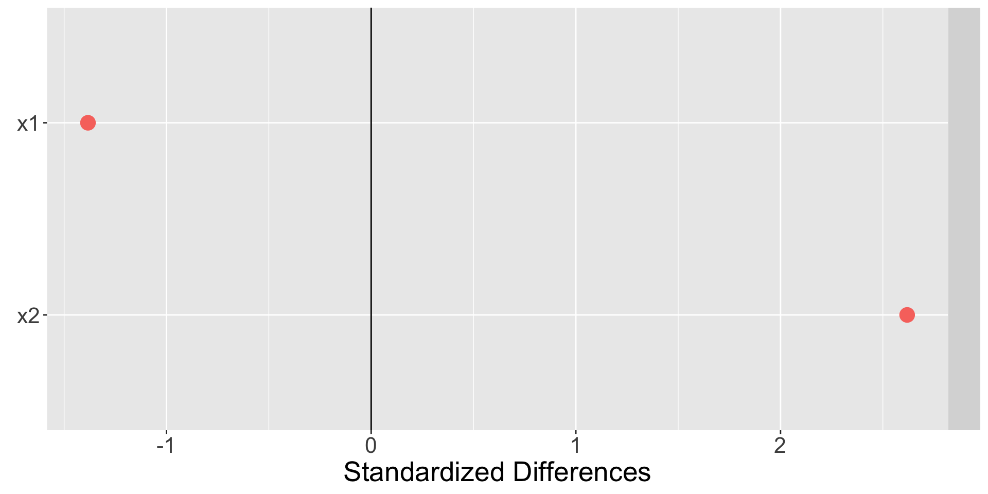
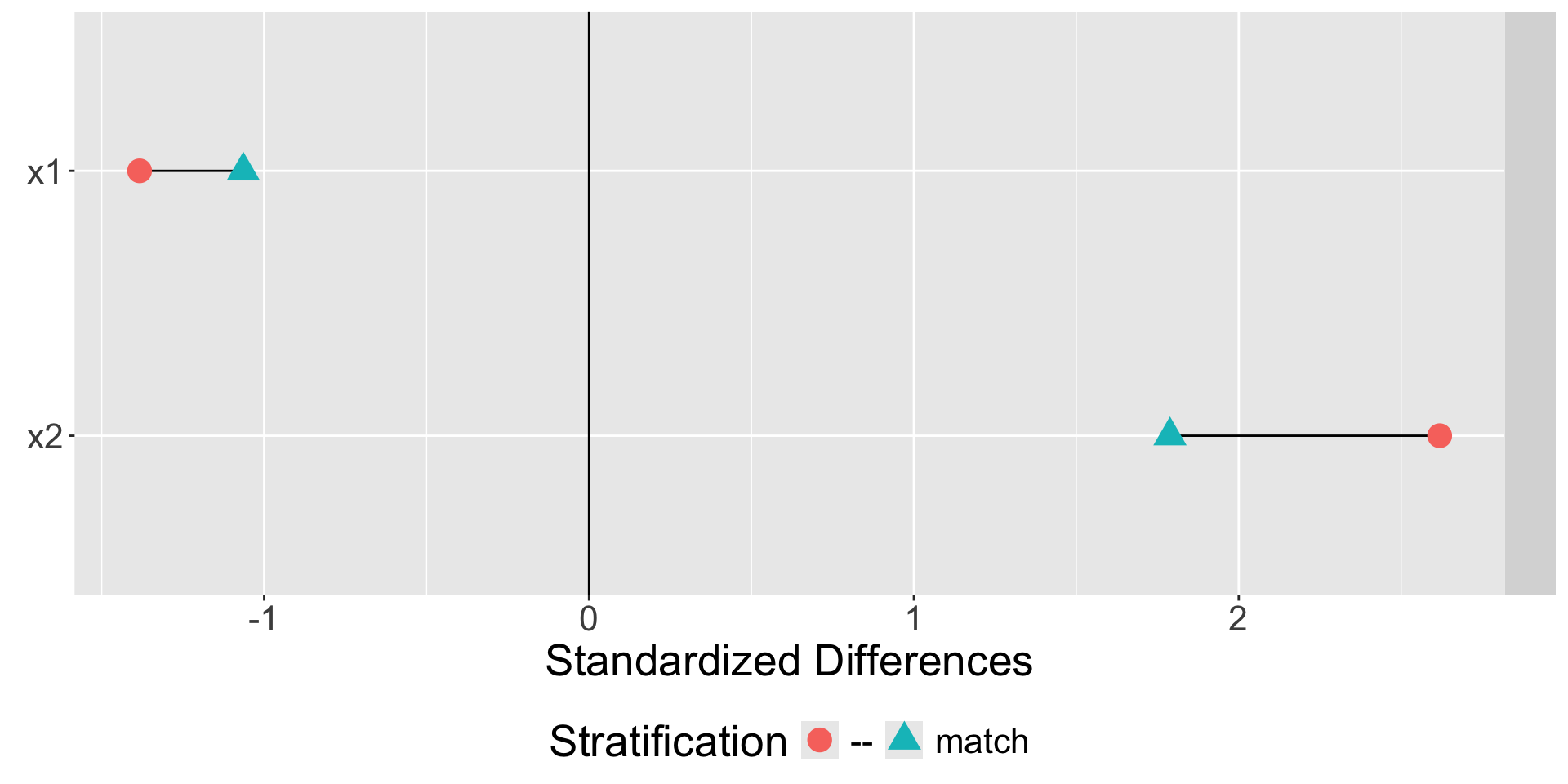
    • Checks balance and ploting the result of balanceTest will produce a Love plot.
#install.packages("RItools")
library(RItools)
baltest <- balanceTest(group ~ x1 + x2, data = d)
baltest
     strata():        --                                       
     stat      Treatment Control adj.diff std.diff    z        
vars                                                           
x1                  1.3     3.5      -2.2     -1.4    -1.8 .   
x2                  5.7     2.2      3.4       2.6     2.6 *   
---Overall Test---
   chisquare df p.value
--       7.1  2   0.028
---
Signif. codes:  0 '***' 0.001 '** ' 0.01 '*  ' 0.05 '.  ' 0.1 '   ' 1 
  • Null hypothesis is balance - we don’t want to reject!
plot(baltest)
  • Now compare the unmatched data to the matched data.
baltest2 <- balanceTest(group ~ x1 + x2 + strata(match), data = d)
print(baltest2, horizontal = FALSE)
$match
   Treatment Control adj.diff std.diff    z sig.
x1       1.3     3.0     -1.7     -1.1 -1.4     
x2       5.7     3.3      2.3      1.8  1.4     

$`--`
   Treatment Control adj.diff std.diff    z sig.
x1       1.3     3.5     -2.2     -1.4 -1.8  .  
x2       5.7     2.2      3.4      2.6  2.6  *  

---Overall Test---
      chisquare df p.value
match       2.0  2   0.368
--          7.1  2   0.028
---
Signif. codes:  0 '***' 0.001 '** ' 0.01 '*  ' 0.05 '.  ' 0.1 '   ' 1 
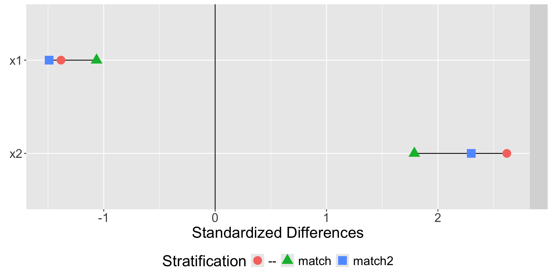
plot(baltest2)

Optimal and Full matching

j:k notation

  • Pair matched data is 1:1 - a single treatment to a single control.
  • 1:2 would mean each treatment member shares two controls.
  • 3:1 means three treatment members share a single control.
  • The optimal match will have all matched sets of size j:k where either j = 1 or k = 1.

Optimal matching

  • Greedy matching matches well on first few values, but can suffer later on, while a sub-optimal early match may improve later matches.
    • Shuffle the data…
  • A optimal match is equivalent to considering all possible matching structures.
  • Optimal is a harder problem but always produces better matches
  • optmatch package uses optimal matching.
  • Distrust any method which uses greedy matching!

1:k or j:1 matching

  • Optimal pair matching useful if sample sizes are close - easy to interpret.
  • Not good if one group is much larger.
    • Loses data
  • 1:k or j:1 matching allows less data loss.

1:k or j:1 matching in optmatch

  • controls argument to pairmatch - # of controls per treated unit
    • 2, 3, 4, etc for 1:k.
    • 1/2, 1/3, 1/4, etc for j:1.
d$match2 <- pairmatch(group ~ x1 + x2,
                      controls = 2, data = d)
d$match2
 [1] 1.2  1.1  <NA> 1.3  1.3  <NA> 1.1  1.2  1.1  1.2  1.3 
summary(d$match2)
Structure of matched sets:
1:2 0:1 
  3   2 
Effective Sample Size:  4 
(equivalent number of matched pairs).
baltest3 <- balanceTest(group ~ x1 + x2 + strata(match2) +
                          strata(match),
                     data = d)
print(baltest3, horizontal = FALSE)
$match2
   Treatment Control adj.diff std.diff    z sig.
x1       1.3     3.7     -2.3     -1.5 -2.0  .  
x2       5.7     2.7      3.0      2.3  2.1  .  

$match
   Treatment Control adj.diff std.diff    z sig.
x1       1.3     3.0     -1.7     -1.1 -1.4     
x2       5.7     3.3      2.3      1.8  1.4     

$`--`
   Treatment Control adj.diff std.diff    z sig.
x1       1.3     3.5     -2.2     -1.4 -1.8  .  
x2       5.7     2.2      3.4      2.6  2.6  *  

---Overall Test---
       chisquare df p.value
match2       4.4  2   0.112
match        2.0  2   0.368
--           7.1  2   0.028
---
Signif. codes:  0 '***' 0.001 '** ' 0.01 '*  ' 0.05 '.  ' 0.1 '   ' 1 
plot(baltest3)

Impossible matches fail

Setting up restrictions on matches that cannot be met produce an error:

pairmatch(group ~ x1 + x2, data = d, controls = 3)
Error in fullmatch.matrix(x = x, min.controls = controls, max.controls = controls, : negative 'omit.fraction' with 'min.controls' >= 2 not permitted

Issues with 1:k or j:1 matching

  • Even with 1:k, can still lose up to \((n_c - k*n_t)\) data.
    • E.g., 10 treatment, 67 controls, 1:6 matching loses 7 controls.
  • Can force bad matches just to meet goal. Flexibility might help.

An example

Treatment Control
5 4
10 5
6
11

An example

Treatment Control
5 4
10 5
6
11

1:2 matching:

Treatment Control
5 4, 5
10 6, 11
  • 6 is a poor match for 10.

An example

Treatment Control
5 4
10 5
6
11

Flexible matched set sizes:

Treatment Control Size
5 4, 5, 6 1:3
10 11 1:1

Fullmatching

  • Allow 1:k or j:1 where k or j can vary per matched set.
d$fullmatch1 <- fullmatch(group ~ x1 + x2, data = d)
summary(d$fullmatch1)
Structure of matched sets:
 1:1 1:5+ 
   2    1 
Effective Sample Size:  3.7 
(equivalent number of matched pairs).
  • Guaranteed to find the best possible match.
  • Best may not be useful: 99:1 and 1:99.
    • Also lowers power (ESS)
  • Instead we set constraints, e.g. all sets between 2:1 and 1:3.
d$fullmatch2 <- fullmatch(group ~ x1 + x2,
                          max.controls = 3,
                          min.controls = 1/2,
                          data = d)
summary(d$fullmatch2)
Structure of matched sets:
1:2 1:3 
  1   2 
Effective Sample Size:  4.3 
(equivalent number of matched pairs).
baltest4 <- balanceTest(group ~ x1 + x2 + strata(fullmatch2) +
                    strata(fullmatch1) + strata(match2) +
                       strata(match), data = d)
print(baltest4, horizontal = FALSE)
$fullmatch2
   Treatment Control adj.diff std.diff    z sig.
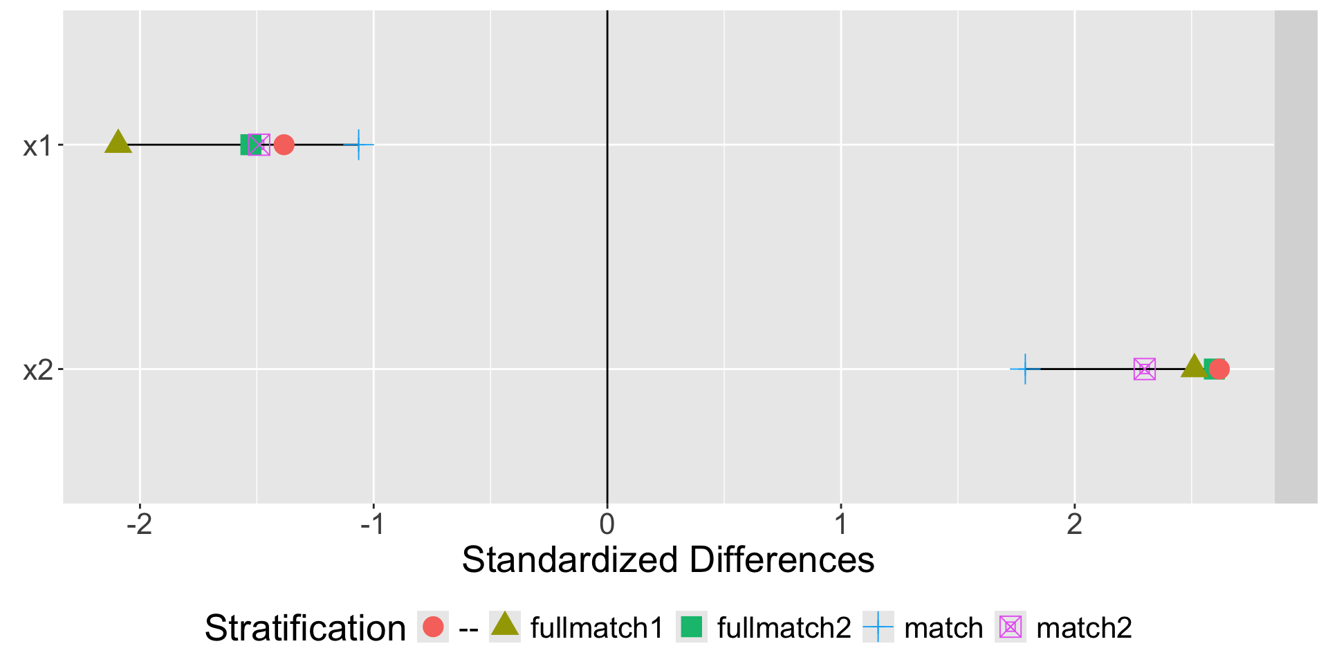
x1       1.3     3.7     -2.4     -1.5 -2.2  *  
x2       5.7     2.3      3.4      2.6  2.3  *  

$fullmatch1
   Treatment Control adj.diff std.diff    z sig.
x1       1.3     4.6     -3.3     -2.1 -1.8     
x2       5.7     2.4      3.3      2.5  1.8     

$match2
   Treatment Control adj.diff std.diff    z sig.
x1       1.3     3.7     -2.3     -1.5 -2.0  .  
x2       5.7     2.7      3.0      2.3  2.1  .  

$match
   Treatment Control adj.diff std.diff    z sig.
x1       1.3     3.0     -1.7     -1.1 -1.4     
x2       5.7     3.3      2.3      1.8  1.4     

$`--`
   Treatment Control adj.diff std.diff    z sig.
x1       1.3     3.5     -2.2     -1.4 -1.8  .  
x2       5.7     2.2      3.4      2.6  2.6  *  

---Overall Test---
           chisquare df p.value
fullmatch2       5.6  2   0.062
fullmatch1       3.3  2   0.189
match2           4.4  2   0.112
match            2.0  2   0.368
--               7.1  2   0.028
---
Signif. codes:  0 '***' 0.001 '** ' 0.01 '*  ' 0.05 '.  ' 0.1 '   ' 1 
plot(baltest4)

Speeding up matching

Distance Matrix

   c1  c2 c3  c4 c5
t1  1 Inf  5 Inf  4
t2  4   2  1   6  4
t3  0   0  5   1  3
  • Each entry represents a distance.
  • 0 represents “identical”, Inf represents never match.
  • The more Inf, the faster matching will run.
  • Built in optmatch, similar notation
m1 <- match_on(group ~ x1 + x2, data = d)
m1
         control
treatment     1     2     3     4     5     6     7     8
       9  2.828 4.186 4.631 4.574 4.495 4.631 4.186 1.809
       10 1.046 2.506 2.828 2.996 3.235 2.828 2.506 0.000
       11 3.525 4.325 5.165 4.436 3.861 5.165 4.325 2.919
  • How do we induce Inf into the distance matrix?

Exact Matching

str(d)
'data.frame':   11 obs. of  4 variables:
 $ group   : num  0 0 0 0 0 0 0 0 1 1 1
 $ x1      : num  2 4 3 5 6 3 4 1 0 1 3
 $ x2      : num  3 2 1 2 3 1 2 4 6 4 7
 $ category: num  0 1 1 0 0 1 0 1 1 0 1
em <- exactMatch(group ~ category, data = d)
as.matrix(em)
       control
treated   1   2   3   4   5   6   7   8
     9  Inf   0   0 Inf Inf   0 Inf   0
     10   0 Inf Inf   0   0 Inf   0 Inf
     11 Inf   0   0 Inf Inf   0 Inf   0
  • More useful than just adding a lot of Inf’s…
  • … because each sub-problem can be considered its own matching problem.
em
$`0`
       control
treated 1 4 5 7
     10 0 0 0 0

$`1`
       control
treated 2 3 6 8
     9  0 0 0 0
     11 0 0 0 0
  • We can combine distance matrices
m1 + em
$`0`
       control
treated     1     4     5     7
     10 1.046 2.996 3.235 2.506

$`1`
       control
treated     2     3     6     8
     9  4.186 4.631 4.631 1.809
     11 4.325 5.165 5.165 2.919
  • This works for distance matricies of any format (from match_on, exactMatch or caliper [which we’ll see in a few slides]).
  • Can be done in a single step as well:
m2 <- match_on(group ~ x1 + x2, data = d, within = em)
m2
$`0`
       control
treated     1     4     5     7
     10 1.046 2.996 3.235 2.506

$`1`
       control
treated     2     3     6     8
     9  4.186 4.631 4.631 1.809
     11 4.325 5.165 5.165 2.919
  • This should be slightly faster than two separate calls.
  • Now, perform matching directly on this distance.
emmatch <- fullmatch(m2, data = d)
summary(emmatch)
Structure of matched sets:
1:1 1:3 1:4 
  1   1   1 
Effective Sample Size:  4.1 
(equivalent number of matched pairs).
emmatch
  1   2   3   4   5   6   7   8   9  10  11 
0.1 1.2 1.1 0.1 0.1 1.1 0.1 1.1 1.1 0.1 1.2 

Calipering

  • For any pairs with large distances, we may want to either
    • Ensure they never match.
      • (Overall match may suffer, but no individual match is terrible.)
    • Speed up calculations by not checking them.
as.matrix(m1)
         control
treatment     1     2     3     4     5     6     7     8
       9  2.828 4.186 4.631 4.574 4.495 4.631 4.186 1.809
       10 1.046 2.506 2.828 2.996 3.235 2.828 2.506 0.000
       11 3.525 4.325 5.165 4.436 3.861 5.165 4.325 2.919
c1 <- caliper(m1, width = 4)
c1
       control
treated 1   2   3   4   5   6   7 8
     9  0 Inf Inf Inf Inf Inf Inf 0
     10 0   0   0   0   0   0   0 0
     11 0 Inf Inf Inf   0 Inf Inf 0
m1 + c1
       control
treated     1     2     3     4     5     6     7     8
     9  2.828   Inf   Inf   Inf   Inf   Inf   Inf 1.809
     10 1.046 2.506 2.828 2.996 3.235 2.828 2.506 0.000
     11 3.525   Inf   Inf   Inf 3.861   Inf   Inf 2.919

Calipering one dimension

  • Sometimes you might want to caliper only one dimension rather than overall distance - e.g. only x1, not the combination of x1 and x2.
  • Two steps process.
    1. Generate a distance matrix for x1 and caliper it (creating a matrix of 0’s and Inf’s).
    2. Generate the distance matrix for x1 and x2 and add it to the caliper’d matrix from step 1.
  • Slightly different result than calipering overall distance.

Combining it all

mm <- match_on(group ~ x1 + x2, data = d,
               within = em, caliper = 4)
mm
$`0`
       control
treated     1     4     5     7
     10 1.046 2.996 3.235 2.506

$`1`
       control
treated   2   3   6     8
     9  Inf Inf Inf 1.809
     11 Inf Inf Inf 2.919
  • Looks like some unmatchable controls.
summary(fullmatch(mm, data = d))
Structure of matched sets:
2:1 1:4 0:1 
  1   1   3 
Effective Sample Size:  2.9 
(equivalent number of matched pairs).

Discussion

  • 3-way trade-off between balance, speed and effective sample size (power).
    • More constraints on j:k leads to more power but is slower.
      • Too few constraints can limit usefulness.
      • May throw away a lot of data, negating power gain.
    • More exact matching or calipering leads to faster but less balanced matches.
      • Too many restrictions can reduce power.
      • Too few restrictions can limit usefulness.
    • Dropping observations leads to more balance matches with lower power.

Example

ECLS data

  • Early Childhood Longitudinal Survey
dim(ecls)
[1] 5429   21
  • Treatment group is catholic school vs public school.
table(ecls$catholic)

   0    1 
4499  930 

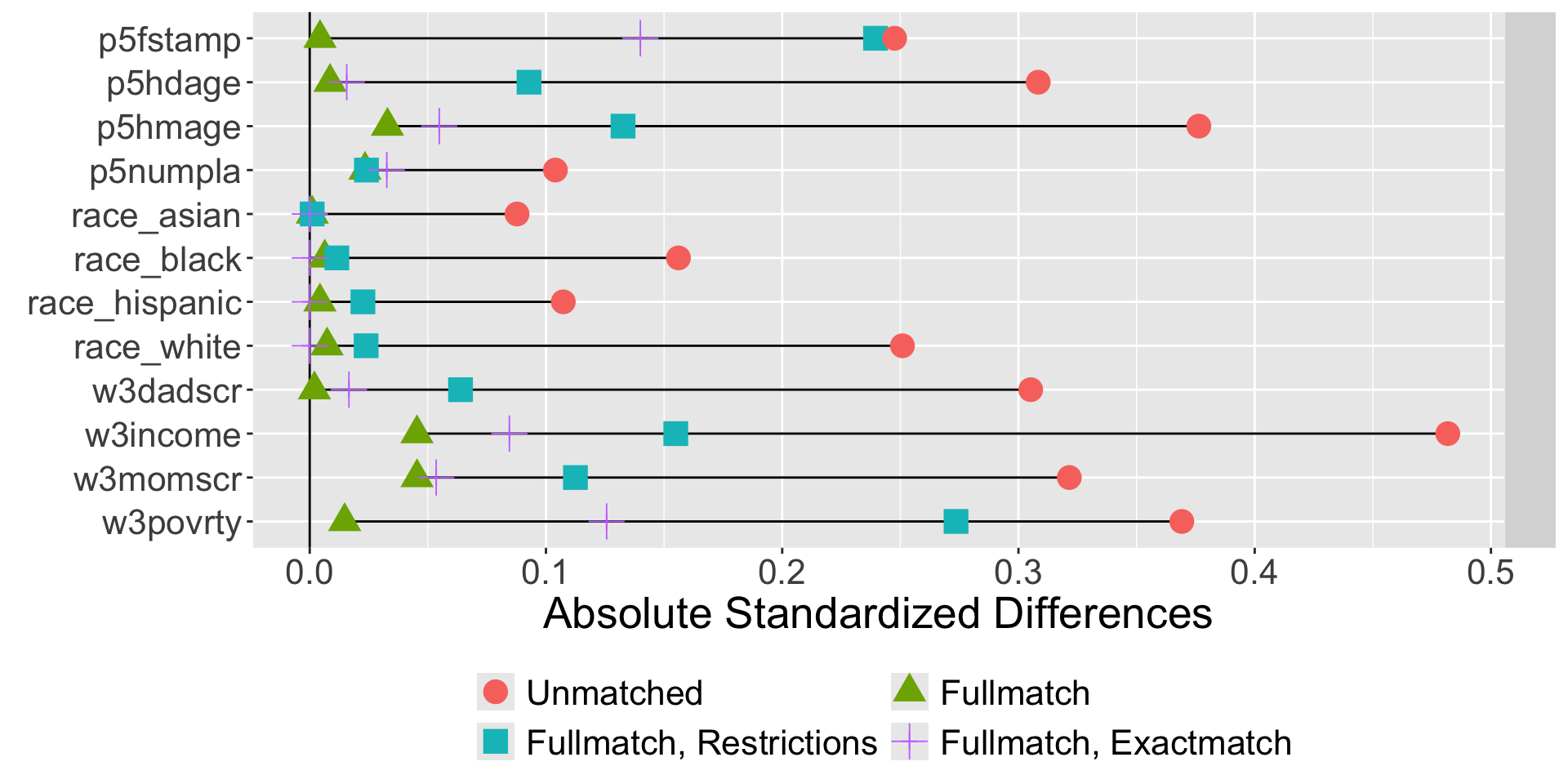
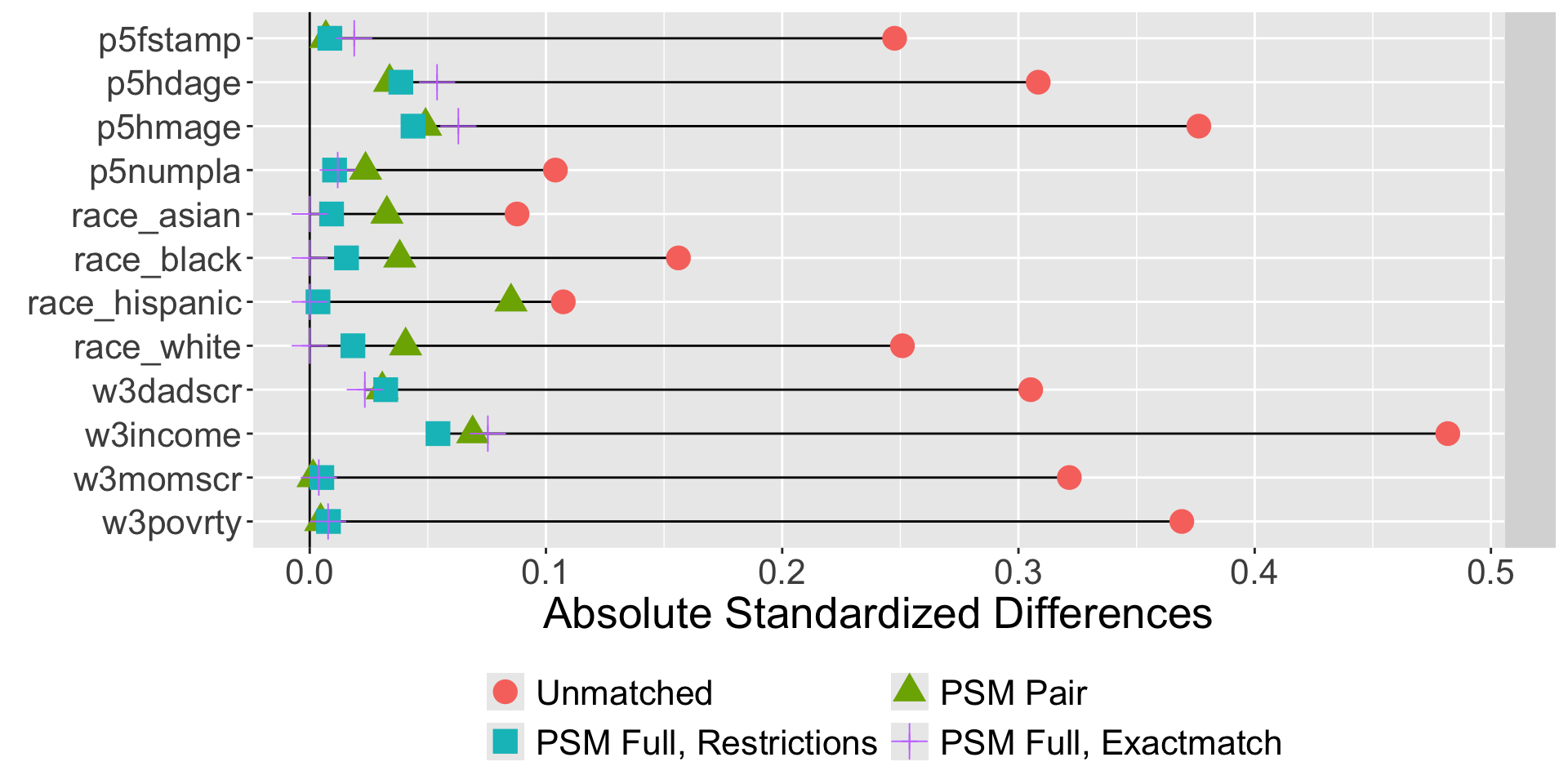
Simulation Results 1

Model Time ESS
Pair match 3.54 930
Pair match (1:2) 5.91 1240
Full match (unres.) 5.87 1342
Full match (restr.) 95.54 1385
Full + Exact 4.65 1347
PS Pair 2.93 930
PS Full 2.70 1313
PSM + Exact 2.58 1305

Simulation Results 2

Simulation Results 3

Simulation Results 4

Simulation Results 5

Model Time ESS Est. Coef p-value
Unmatched NA NA -1.48 <.001
Pair match 3.54 930 -1.51 <.001
Pair match (1:2) 5.91 1240 -1.68 <.001
Full match (unres.) 5.87 1342 -1.49 <.001
Full match (restr.) 95.54 1385 -1.48 <.001
Full + Exact 4.65 1347 -1.49 <.001
PS Pair 2.93 930 -1.59 <.001
PS Full 2.70 1313 -1.48 <.001
PSM + Exact 2.58 1305 -1.48 <.001

Other Matching Methods

  • quickmatch - Generalized Full Matching, fast & more than two groups
  • cem - Coarsened Exact matching, bins continuous variables and uses Exact matching
  • The MatchIt package in R handles these and other forms of matching
    • Including optmatch! (But the actual optmatch package allows more flexiblity).

References

Austin, Peter C. 2011. “An Introduction to Propensity Score Methods for Reducing the Effects of Confounding in Observational Studies.” Multivariate Behavioral Research 46 (3): 399–424.
Bowers, Jake, Mark Fredrickson, Ben Hansen, and Josh Errickson. 2023. RItools: Randomization Inference Tools. https://CRAN.R-project.org/package=RItools.
Hansen, Ben B, Mark Fredrickson, Josh Errickson, Josh Buckner, and Adam Rauh. 2023. Optmatch: Functions for Optimal Matching. https://CRAN.R-project.org/package=optmatch.
Hansen, Ben B., and Stephanie Olsen Klopfer. 2006. “Optimal Full Matching and Related Designs via Network Flows.” Journal of Computational and Graphical Statistics 15 (3): 609–27.